
On this page 12 sections
- Preface
- Chapter 1 · Why is the effect of advertising so hard to see?
- Chapter 2 · What does a reported conversion actually record?
- Chapter 3 · What can an attribution model tell you, and what can't it?
- Chapter 4 · Why do observational ad measurements overstate effects?
- Chapter 5 · How do you measure what an ad caused?
- Chapter 6 · How should budget follow evidence?
- Chapter 7 · How do attribution, experiments and models fit together?
- Chapter 8 · Can an AI analyst tell credit from cause?
- Conclusion · Twelve propositions
- Appendices
- Practical guides
Abstract
Every advertising report hands out credit. A platform says its ads drove 300 purchases, an attribution model says Search earned 75% of last month's orders, and a dashboard ranks channels by return on ad spend. None of these numbers says what the advertising caused, meaning how many sales would have disappeared if the ads had not run. This book is about the distance between those two quantities.
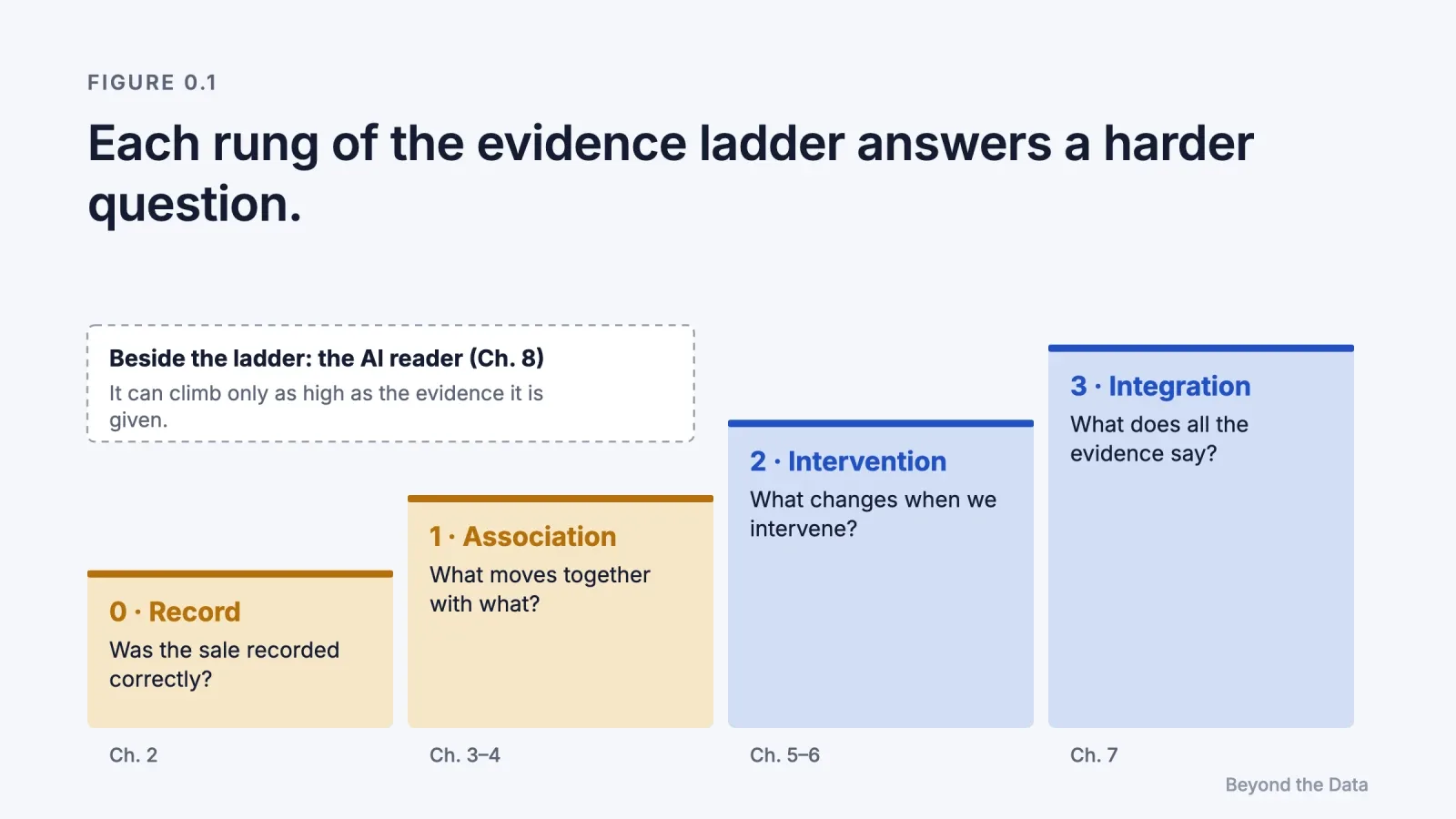
The book assembles the evidence on that distance into one framework, the evidence ladder. Each rung answers a harder question. Rung 0 asks whether a sale was recorded correctly. Rung 1 asks what moves together with what. Rung 2 asks what changes when we intervene. Rung 3 asks what all of the evidence says when it is read together. Attribution models, platform reports and dashboards live on the lower rungs. Experiments live on rung 2. Media mix models and calibrated systems try to reach rung 3.
The evidence comes from controlled experiments run on the largest advertising platforms, from meta-analyses that cover thousands of campaigns, and from the platforms' own documentation. Three findings recur. Advertising effects are real but small relative to the noise in sales. Observational methods tend to overstate them, sometimes by a factor of ten or more. And the credit that attribution assigns behaves by rules that have no causal meaning: when channels reinforce each other, their separate causal effects add up to more than 100% of the sales they jointly produce, so there is no single natural division of credit; a causal split exists only under stated assumptions about how interactions are shared.
The final chapter adds an original test. Because many marketers now ask AI assistants to read their advertising data, we gave six measurement traps to two families of language models. With the evidence visible, both reached the right decision in almost every case. Their characteristic slip was a different one: when a test covered half of a store, some answers compared the half-store loss with whole-store spend (35 of 120 in a replication). When the slip would have changed the decision, it fell to 6 of 120, and no answer switched the channel off.
The book ends with twelve numbered propositions, each tied to a chapter and its sources.
How to read this book
The book is written to be read in three layers.
- Skim layer (5 minutes). Read the twelve propositions at the end. Each one stands on its own.
- Decision layer (30 minutes). Every chapter opens with its question, a short answer of about fifty words, and a box of key findings. Reading only those gives the full argument.
- Evidence layer (about 80 minutes). The body of each chapter shows the studies, their designs and their numbers, and closes with the limit that leads to the next chapter.
Every factual claim carries an evidence label:
| Label | Meaning |
|---|---|
| [Experiment] | Randomised controlled trial or field experiment |
| [Observational] | Estimated from data without random assignment |
| [Model] | Output of a statistical or simulation model |
| [Platform] | Statement by an advertising platform about its own product |
| [Experiment vs observational] | A study that compares an experiment's result with observational estimates for the same campaigns |
| [Analytical] | A result derived mathematically rather than from data |
| [Methodological review] | A review of when a method can be trusted |
| [Textbook principle] | An established principle in a field's textbooks |
| [Industry survey] | A survey of marketers or companies; it shows what is done, not what works |
| [Benchmark] | Language models' score on a standard set of tasks |
| [Our test] | The test run for this book (Chapter 8, Appendix D) |
| [Our reading] | Our inference from the sources, not a finding of any study |
The evidence ladder
| Rung | Question | Typical methods | Chapters |
|---|---|---|---|
| 0 · Record | Was the sale recorded correctly? | Tracking, attribution windows, consent, modelled conversions | 2 |
| 1 · Association | What appears together with what? | Attribution models, dashboards, before-and-after comparisons | 3, 4 |
| 2 · Intervention | What changes when we change something? | Holdouts, ghost ads, geo experiments, synthetic controls | 5, 6 |
| 3 · Integration | What does all the evidence say together? | Media mix models, calibration, triangulation | 7 |
| Beside the ladder · Reader | Which rung can an AI analyst reach? | Language models reading reports | 8 |
Chapter 1 explains why the ladder is needed at all: the effect of advertising is a difference between two worlds, and only one of them can be observed.
The ladder borrows its shape from two older ideas, Judea Pearl's ladder of causation (association, intervention, counterfactuals) and the hierarchy of evidence used in medicine. It is not identical to either. Rung 0 has no counterpart in Pearl's ladder because advertising data, unlike most scientific data, is recorded by an interested party. The ladder orders the scope of the question, not the strength of the evidence: a method on a higher rung asks a broader question, but its answer is not always more reliable.
Chapter map
| # | Question | Short answer |
|---|---|---|
| 1 | Why is the effect of advertising so hard to see? | The effect is the gap between sales with and without the ads. It is small, sales are noisy, and ads go to people who were likely to buy anyway. |
| 2 | What does a reported conversion actually record? | A recorded conversion can be missing, counted twice, or modelled. The platform that sold the ad also grades it. |
| 3 | What can an attribution model tell you, and what can't it? | Attribution divides credit by a rule. When channels reinforce each other, their causal effects add up to more than 100%, so there is no single natural split. |
| 4 | Why do observational ad measurements overstate effects? | Targeting and user activity make exposed people different from unexposed ones. Across hundreds of experiments, observational methods miss the experimental answer by large margins. |
| 5 | How do you measure what an ad caused? | Randomise who can see the ad, then compare. Holdouts, ghost ads and geo experiments are the main designs, each with a cost and a blind spot. |
| 6 | How should budget follow evidence? | Follow the marginal return, not the average. Saturation, delay and synergy all move the margin away from what reports show. |
| 7 | How do attribution, experiments and models fit together? | Attribution gives daily direction, experiments give ground truth, models spread it across channels. Calibration connects them. |
| 8 | Can an AI analyst tell credit from cause? | In our test, yes when the evidence is visible. The typical slip was arithmetic scale, not causal confusion. |
Original contributions
- The evidence ladder. It orders measurement methods into four rungs by the question they ask; the record rung has no counterpart in Pearl's ladder. (This page)
- Totals above 100%. It carries the epidemiological principle that attributable fractions can sum to more than 100% (Rothman) over to attribution. (Chapter 3)
- The self-grading platform. It treats a platform measuring the ads it sold as a distinct type of error. (Chapter 2)
- A triangulation routine. It combines attribution, experiments and media mix models into one operating routine through calibration. (Chapter 7)
- An AI analyst test. It tests whether language models can tell credit from cause, using cases with known answers. (Chapter 8, Appendix D)
- Evidence labels and twelve propositions. Every claim shows the kind of evidence behind it, and the argument is gathered into twelve propositions, each tied to a chapter. (Conclusion)
What this book does not measure
The evidence in this book comes mostly from online advertising and from experiments that last days or weeks. It measures what advertising adds to sales within that window. Four things fall outside it.
- Long-term brand effects. Advertising can build memory, preference and pricing power over months or years. Short tests do not see this. The meta-analysis in Chapter 1 found long-run elasticities about twice the short-run ones, so a test that ends early tends to understate the total effect.
- Reach beyond the targeted audience. User-level experiments run inside the audience a platform has already chosen. The value of reaching people who are not yet thinking of buying lies largely outside their view.
- Creative. An experiment says what one ad did in one period. It does not say why that ad worked or what a better ad would have done.
- What has not been tested. A missing experiment is missing evidence. It is not evidence that a channel does nothing.
[Our reading] When a channel's purpose is long-term, keep the paused regions under observation for several weeks after the test ends, and read the test result as likely to understate the total effect.
Conflict of interest
The author is a co-founder of Meerkads, a company that builds advertising analytics software, including tools that let AI assistants read advertising data. The book does not describe or recommend any Meerkads product. The Practical guides page at the end of the book links, chapter by chapter, to practical guides on the Meerkads blog; the chapters themselves carry no such links. Several sources are written by employees of advertising platforms or use platform data; each such case is noted where it is cited, because access to experimental advertising data is in practice only possible from inside a platform.
Preface
How do you read advertising data correctly? In a team that had worked with advertising data for many years, that was the question we chased most. When we could not find a tool that gave us that reading, and the meaningful insights that follow from it, we built our own system around our needs. We knew what we needed, or at least we thought we did.
Along the way, one question stayed with me: how could I go beyond what we already had? I believed that if I could reach more data, I would get more meaningful answers.
I started researching that question. The research first became blog posts, then kept growing. I never thought it would turn into a book. It moved forward through long rounds of questions, answers and debate with an AI assistant.
The book orders measurement methods on a ladder by the question each one can answer. When channels reinforce each other, their separately measured effects add up to more than 100%, so there is no single natural split; a sale can be divided among channels only under stated assumptions. The book treats a platform measuring the results of the ads it sells as a separate kind of error. It shows how attribution, experiments and models work together, and finally tests whether AI can make these distinctions. The source of every number in the book was opened and read; the one figure taken from a secondary source says so where it appears.
I set out looking for more data; the work carried me from the quantity of data to evidence and cause. The numbers we thought we understood were not saying what we thought.
Edip Ali Avcıbaşı, November 2026
Chapter 1
Why is the effect of advertising so hard to see?
Key findings
- Across 56 studies and 751 estimates, a 1% increase in advertising raises sales by about 0.12% in the short run and 0.24% in the long run (Sethuraman et al., 2011). [Observational, meta-analysis]
- For 288 consumer brands on US television, the estimated effects were smaller still, and for more than 80% of brands the last dollar of TV advertising lost money (Shapiro et al., 2021). [Observational]
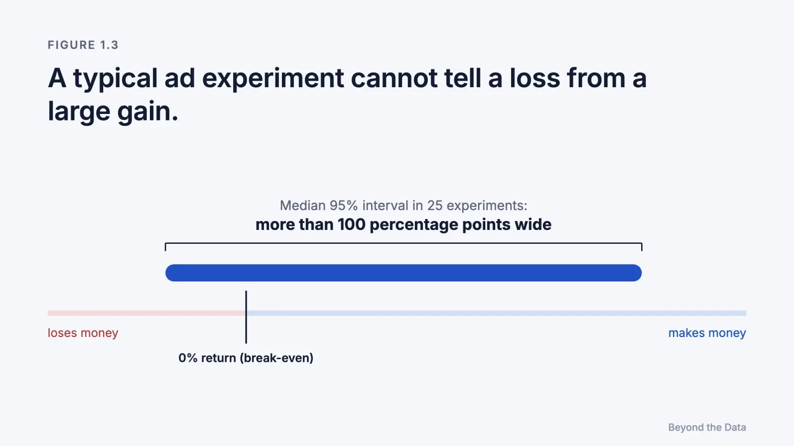
- In 25 large online experiments, the median 95% confidence interval for return on investment was more than 100 percentage points wide (Lewis & Rao, 2015). [Experiment]
- A conclusive experiment can require more than 10 million person-weeks of data (Lewis & Rao, 2015). [Experiment]
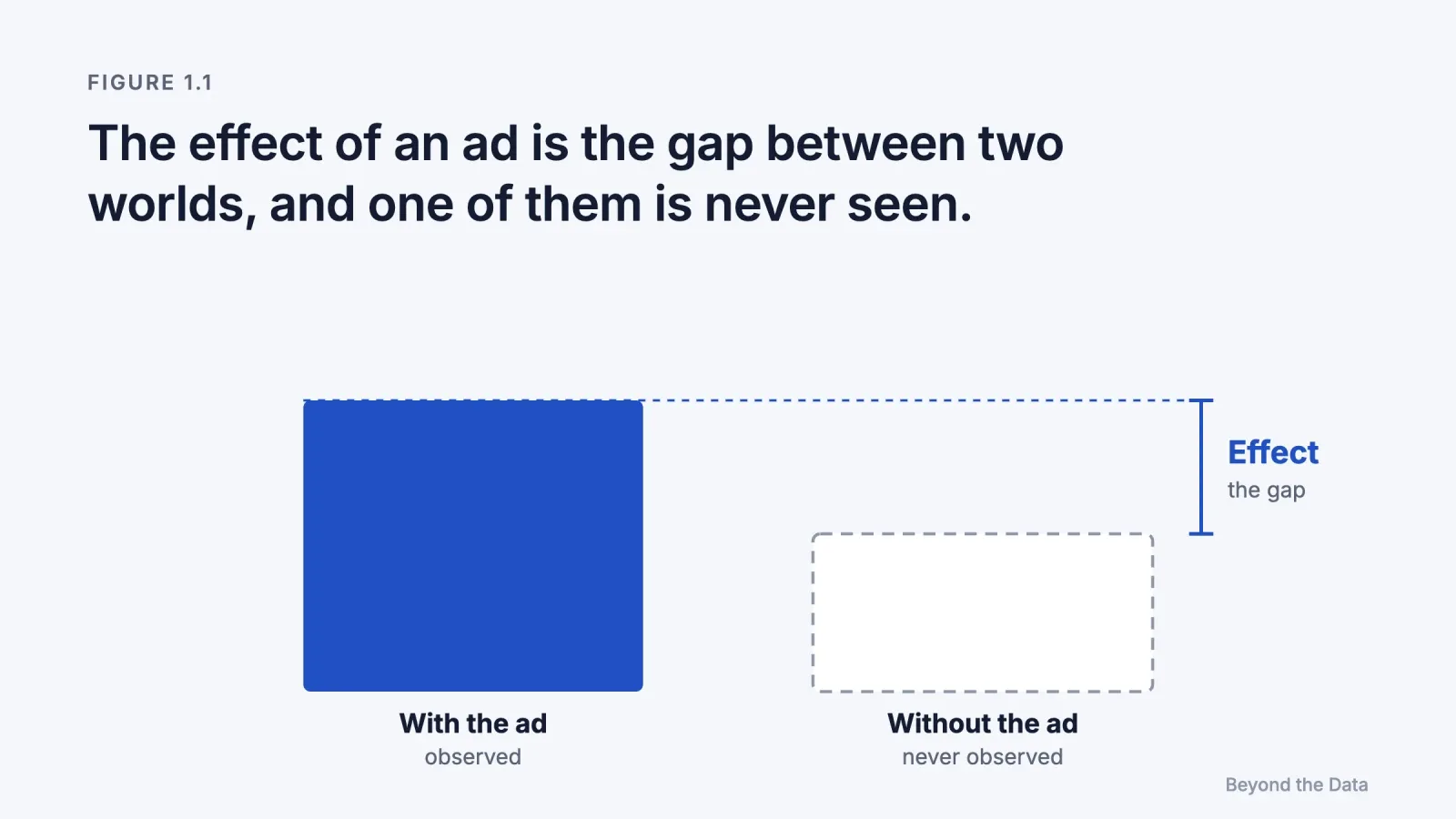
Short answer. The effect of an ad is the difference between the sales that happened and the sales that would have happened without it. The second number is never observed. It has to be inferred, and the inference is hard for three reasons: the effect is small, individual sales are very noisy, and ads are shown to people who were already likely to buy.
What exactly is "the effect" of an ad?
The causal effect of an advertisement is the difference between what a customer did after seeing it and what the same customer would have done without seeing it. Statisticians call the two quantities potential outcomes (Imbens & Rubin, 2015). For any one person, only one of them is ever observed. A customer who saw the ad and bought cannot also be observed not seeing it.
Every method in this book is a way of estimating the missing outcome. Some estimate it well, some badly, and some do not try at all. A report that counts purchases after an ad click estimates nothing about the missing outcome. It records that a click and a purchase happened in sequence.
This is why the book separates two words. Credit is the share of a sale that a report assigns to an ad. Cause is the share of a sale that would disappear if the ad were removed. Credit is a bookkeeping choice and is always available. Cause is a fact about the world and is never directly visible.
How large are advertising effects?
Smaller than most dashboards suggest. Marketing scientists express the effect of advertising as an elasticity: the percentage change in sales for a 1% change in advertising.
| Study | Scope | Finding | Evidence |
|---|---|---|---|
| Sethuraman, Tellis & Briesch (2011) | 56 studies, 751 short-term and 402 long-term elasticities, 1960–2008 | Average elasticity 0.12 short term, 0.24 long term; down from 0.22 and 0.41 in an earlier meta-analysis; declining over time | Observational, meta-analysis |
| Lodish et al. (1995) | 389 split-cable TV experiments | Raising budgets relative to competitors does not, in general, raise sales. For 89 established products the average elasticity was 0.05, and 33% of estimates were significant at a lenient one-tailed 20% level (as summarised by Shapiro et al.) | Experiment |
| Shapiro, Hitsch & Tuchman (2021) | 288 consumer packaged goods brands, US TV | Elasticities far smaller than earlier literature, many not significant; marginal ROI negative for over 80% of brands; overall ROI positive for about one third | Observational |
Two things follow. First, a typical advertiser who raises spend by 10% should expect sales to rise by about 1%, often less. Second, the effect has been shrinking or was overstated in earlier work, or both. Shapiro and colleagues argue that published estimates were selected for being large and significant, while their own sample was not.
None of this says advertising does not work. Shapiro's data show that for about one third of brands the advertising they already run is profitable overall, even when the next dollar is not. It says that the effect is a small signal that has to be separated from a large background.

Why can't we just compare buyers who saw the ad with buyers who didn't?
Because the two groups were different before the ad was shown. Online advertising is targeted on purpose. Platforms show ads to people whose behaviour predicts a purchase: recent visitors, people who searched for the product, people similar to past buyers. If the ad then "converts" at four times the rate of the general population, most of that gap existed before the ad.
Lewis and Rao (2015) describe this as the core weakness of observational methods: selection, created by targeting, is large compared with the effect being measured. A second bias is subtler. Lewis, Rao and Reiley (2011) found that people who are very active online on a given day are both more likely to see an ad and more likely to do everything else, including visiting the advertiser's site. In one of their Yahoo experiments, visits to Yahoo jumped among exposed users, but the same jump appeared in the placebo group that saw an unrelated ad. They called it activity bias. [Experiment]
Chapter 4 shows how large these biases become in practice.
Why is sales data so noisy?
Because a single customer's purchases vary enormously compared with the cost of reaching that customer. Lewis and Rao (2015) ran 25 field experiments with major US retailers and brokerages, covering $2.8 million of online advertising. In their data, the standard deviation of a customer's sales was typically about ten times its mean. Against that variation, an ad that costs a few cents per person and lifts the average by a fraction of a percent is almost invisible. [Experiment]
The consequences are concrete:
- The median 95% confidence interval for ROI in their experiments was more than 100 percentage points wide. An honest result often reads "somewhere between losing money and doubling it".
- A conclusive experiment could require more than 10 million person-weeks of observation, which is beyond the reach of most advertisers.
They called this "the unfavorable economics of measuring the returns to advertising". It is the main reason why so much measurement relies on cheaper methods that do not use random assignment, and therefore why so much measurement is biased.
What does this mean for an advertiser?
[Our reading] Three practical consequences follow from the evidence above.
- A large reported return is more likely to be wrong than a small one. Given typical elasticities, a channel reporting a tenfold return on ad spend is more likely to be capturing selection than causing sales.
- A single week of data rarely settles anything. Sales noise means that week-to-week swings in a channel's reported performance mostly reflect noise and seasonality.
- The missing outcome has to be estimated deliberately. If no method in the reporting stack tries to estimate what would have happened without the ads, the stack is reporting credit, not cause.
The limit of this chapter
This chapter treated the observed numbers as correct and asked why they do not show causes. Before going further, we have to check that assumption. The numbers in an advertising report are recorded by tracking systems, filtered by consent, and sometimes estimated by models. Chapter 2 asks what a reported conversion actually records.
References
- Imbens, G. W., & Rubin, D. B. (2015). Causal Inference for Statistics, Social, and Biomedical Sciences. Cambridge University Press. doi:10.1017/CBO9781139025751
- Lewis, R. A., & Rao, J. M. (2015). The unfavorable economics of measuring the returns to advertising. Quarterly Journal of Economics, 130(4), 1941–1973. doi:10.1093/qje/qjv023
- Lewis, R. A., Rao, J. M., & Reiley, D. H. (2011). Here, there, and everywhere: Correlated online behaviors can lead to overestimates of the effects of advertising. Proceedings of WWW 2011, 157–166. doi:10.1145/1963405.1963431
- Lodish, L. M., Abraham, M., Kalmenson, S., Livelsberger, J., Lubetkin, B., Richardson, B., & Stevens, M. E. (1995). How T.V. advertising works: A meta-analysis of 389 real world split cable T.V. advertising experiments. Journal of Marketing Research, 32(2), 125–139. doi:10.2307/3152042
- Sethuraman, R., Tellis, G. J., & Briesch, R. A. (2011). How well does advertising work? Generalizations from meta-analysis of brand advertising elasticities. Journal of Marketing Research, 48(3), 457–471. doi:10.1509/jmkr.48.3.457
- Shapiro, B. T., Hitsch, G. J., & Tuchman, A. E. (2021). TV advertising effectiveness and profitability: Generalizable results from 288 brands. Econometrica, 89(4), 1855–1879. doi:10.3982/ECTA17674
Chapter 2
What does a reported conversion actually record?
Key findings
- After Apple's App Tracking Transparency (ATT) framework, the share of trackable Apple traffic in the US fell from 73% to 22% (Kraft et al., 2023). [Observational]
- Since November 2023, Google Analytics 4 offers only data-driven and last-click attribution; first click, linear, time decay and position-based were removed (Google, 2026). [Platform]
- From 12 January 2026, Meta's Ads Insights API no longer returns 7-day and 28-day view-through windows (Meta, 2025). [Platform]
- When platforms report their own results, their totals can exceed the store's revenue, because each platform credits itself for the same sale. [Our reading, illustrated below]
Short answer. A reported conversion is a claim that a sale followed an ad within a chosen time window. The claim can be wrong in three ways: the sale is missing because it could not be tracked, the sale is counted by more than one platform, or the sale was estimated by a model rather than observed. In every case, the platform that sold the ad also decides how the ad is scored.
What is a conversion, in a platform's report?
A conversion in an advertising report is a recorded event, such as a purchase, that the platform links to a person who saw or clicked one of its ads within an attribution window. The definition has three moving parts: what counts as the event, how the link to a person is made, and how long the window is. Change any one of them and the number changes, although nothing about the customers has changed.
This chapter is about rung 0 of the evidence ladder: whether the recorded number is a faithful record at all. A perfect record would still say nothing about cause. An imperfect record makes every later step worse.
Error 1: How do sales go missing?
Sales go missing when the link between an ad and a buyer cannot be observed. The largest single change in recent years was Apple's ATT framework, introduced in 2021, which requires apps to ask permission before tracking users across other companies' apps and websites.
Kraft, Skiera and Koschella (2023) studied billions of ad impressions across eight countries. In the US, the share of Apple traffic that could still be tracked fell from 73.05% to 22.15%, a drop of about 70%. Opt-in rates ranged from 18.18% to 44.65% depending on the country. [Observational]
For a platform, a sale it cannot link to an ad does not exist in the report. Two things follow. Reported conversions fall even when real sales do not. And channels whose buyers are harder to track, such as video and mobile apps, look weaker than channels whose buyers arrive through a tracked click.

Error 2: How can one sale be counted twice?
Each platform sees only its own ads. If a customer saw an ad on Meta, clicked a Google ad later, and then bought, both platforms can claim the sale in good faith. Neither knows about the other.
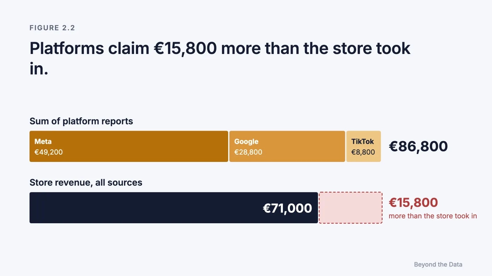
A simple check exposes this. Add up the revenue each platform reports and compare it with the revenue the store actually recorded.
| Source | Revenue reported | Note |
|---|---|---|
| Meta | €49,200 | Platform's own report |
| Google Ads | €28,800 | Platform's own report |
| TikTok | €8,800 | Platform's own report |
| Sum of platform reports | €86,800 | |
| Store revenue (all sources) | €71,000 | Includes sales no ad touched |
Illustrative example used in the test in Chapter 8.
The platforms together claim €15,800 more than the store took in, and the store figure includes organic and direct sales that no platform should claim. So the overlap is at least €15,800 and probably much larger. [Our reading] When the sum of platform claims exceeds the store's total, the individual return-on-ad-spend figures cannot be compared across platforms, because each was computed on a different and overlapping share of the same sales.
Error 3: What is a modelled conversion?
When a sale cannot be tracked, platforms increasingly estimate it. Google's data-driven attribution, the default for most conversion actions in Google Ads, assigns credit by comparing the paths of customers who converted with those who did not (Google, 2026). Meta's incremental attribution, introduced in 2025, uses a model to estimate which conversions were caused by an ad. Meta reports that it delivers 24% more incremental conversions than standard attribution (Meta, 2026). [Platform]
Modelled numbers are not wrong by nature. But they are a different kind of number. A tracked conversion records an event. A modelled conversion is an estimate of an event, made with a method the advertiser cannot inspect.
Who grades the ad?
The platform that sells the ad also measures its result. It chooses the default attribution model, the default window, the treatment of views versus clicks, and how missing data is modelled. We call this self-grading. [Our reading]
Self-grading is not a claim of bad faith. Platforms have the best data about their own ads, and some of the most rigorous studies in this book were made possible by platform data. The problem is structural: the party with the most to gain from a high number controls the definition of the number.
Recent changes illustrate how much the definition matters:
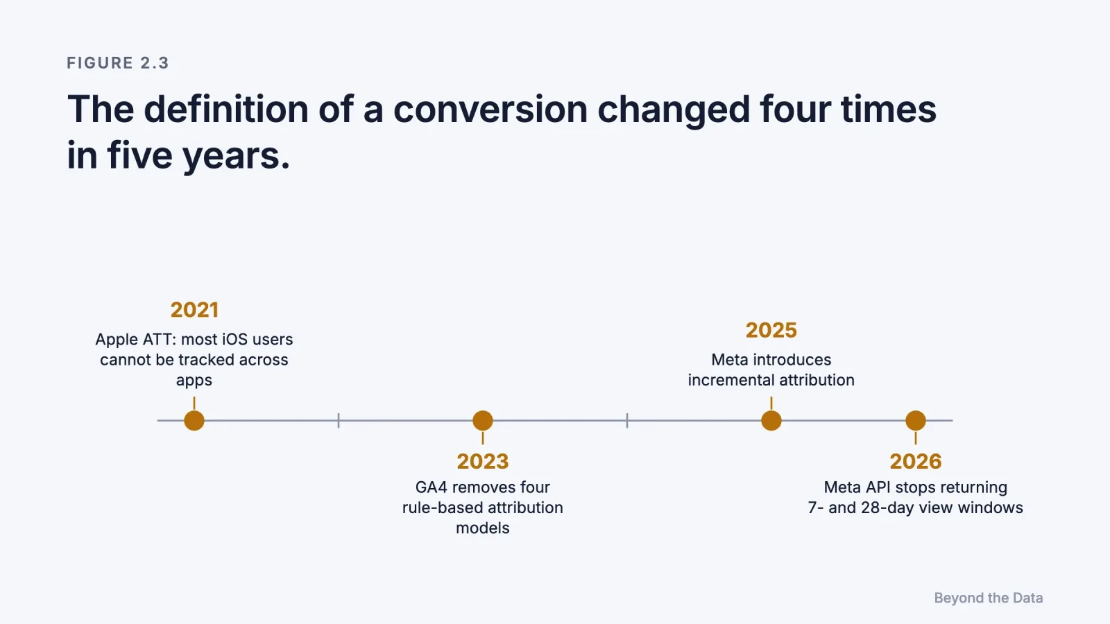
| Year | Change | Source |
|---|---|---|
| 2021 | Apple ATT: most iOS users not trackable across apps | Kraft et al. (2023) |
| 2023 | Google removes four rule-based models from GA4; Google Ads keeps last click and data-driven | Google (2026) |
| 2025 | Meta introduces incremental attribution | Meta (2026) |
| 2026 | Meta API stops returning 7-day and 28-day view windows | Meta (2025) |
Each change altered reported conversions for the same advertising. Advertisers who compare this year's numbers with last year's are often comparing two different definitions.
There is also a deeper incentive problem. Berman (2018) shows with a game-theoretic model that last-touch attribution encourages publishers to over-supply impressions and often lowers advertisers' profit. The scoring rule does not just describe the outcome. It shapes behaviour, including the behaviour of bidding algorithms that are trained on the rule's output. [Model]
What should an advertiser check first?
- Reconcile to the store. Every month, compare the sum of platform-reported revenue with store revenue from all sources. If the sum is close to or above the store total, treat platform ROAS as credit, not as cause.
- Freeze the definitions. Record the attribution model, window and view settings used for each report. A trend is only meaningful if the definition did not change underneath it.
- Separate observed from modelled. Where the platform reports modelled conversions, note them separately from tracked ones.
- Name the grader. For each number in a report, note who produced it. A number produced by the seller of the ad is a platform statement, not independent evidence.
The limit of this chapter
Suppose every sale were recorded once, correctly, and linked to every ad the buyer saw. The record would still show only which ads appeared before which sales. It would not show which sales the ads caused. Turning that record into credit is the job of attribution models, and Chapter 3 asks what those models can and cannot tell us.
References
- Berman, R. (2018). Beyond the last touch: Attribution in online advertising. Marketing Science, 37(5), 771–792. doi:10.1287/mksc.2018.1104
- Google. (2026). About attribution models; About data-driven attribution (Google Ads Help 6259715, 6394265); Attribution models in Google Analytics (Analytics Help 10596866). Accessed 13 November 2026.
- Kraft, L., Skiera, B., & Koschella, T. (2023). Economic impact of Apple's App Tracking Transparency framework. Proceedings of the European Marketing Academy (EMAC).
- Meta. (2025, October 16). Ads Insights API metric availability updates. Meta for Developers Blog.
- Meta. (2026, January 28). Fourth quarter 2025 earnings conference call transcript. [Platform; company statement about its own product]
Chapter 3
What can an attribution model tell you, and what can't it?
Key findings
- Display advertising raises searches for the advertised brand by 30–45% (Lewis & Nguyen, 2015). [Experiment]
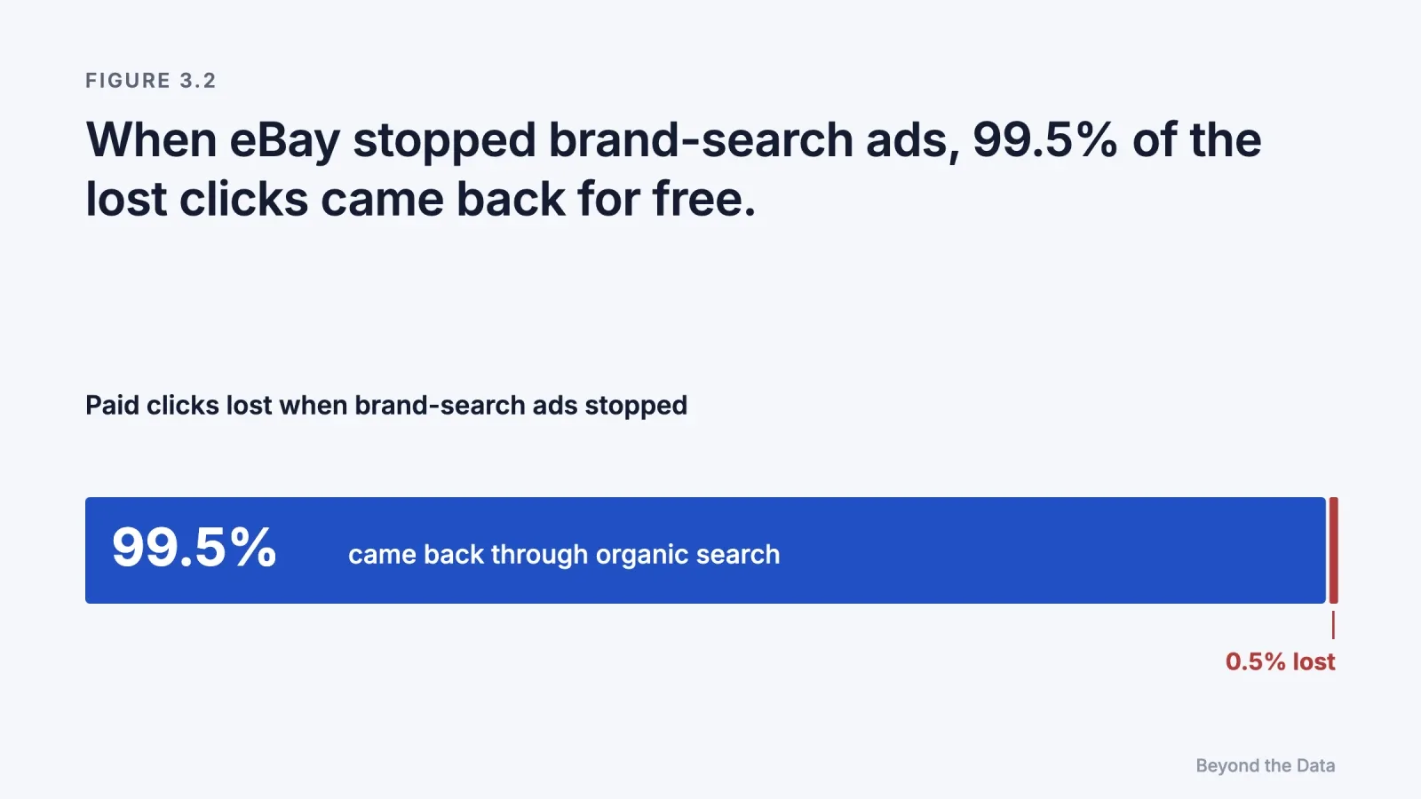
- When eBay switched off brand-keyword search ads, 99.5% of the lost paid clicks came back through organic search (Blake et al., 2015). [Experiment]
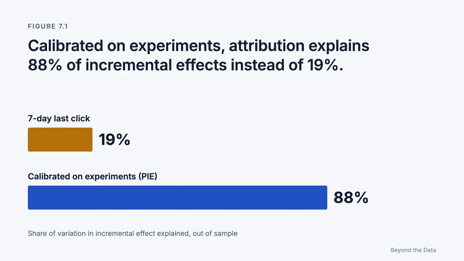
- Across 2,226 Meta experiments, 7-day last-click attribution explained 19% of the variation in incremental conversions per dollar; a model calibrated on experiments explained 88% (Gordon et al., 2026). [Experiment]
- In epidemiology, the fractions of disease attributable to different causes have no upper limit and can sum to well over 100% (Rothman, 2002). [Textbook principle]
Short answer. An attribution model divides the credit for a sale among the ads a customer encountered before buying. Every model forces the shares to add up to exactly 100%. Causal effects do not obey that rule: when channels reinforce each other, the sales lost by removing each channel add up to more than 100%, and when they compete for the same buyers, to less. So the division can describe the customer journey, but it cannot tell you what each channel caused.
What is an attribution model?
An attribution model is a rule that divides the credit for a sale among the ads and channels a customer encountered before buying. Last click gives all credit to the final touch. Linear divides it equally. Data-driven models estimate each channel's share from the paths of past customers.
| Model | How it assigns credit | What it hides |
|---|---|---|
| Last click | All to the final click | Channels that created demand earlier; it inflates brand search and retargeting |
| First click | All to the first touch | Steps that closed the sale |
| Linear | Equal shares | Which touch actually mattered |
| Time decay | More to touches near the sale | Early touches in long decisions |
| Position-based | Fixed shares to first and last, remainder to the middle | That the shares are arbitrary |
| Data-driven (Shapley, Markov) | From the association between a touch and conversion across many paths | That the association is still a correlation: it does not ask whether the sale would have happened without the touch |
Platforms have narrowed the choice. Google Analytics 4 removed first click, linear, time decay and position-based models in November 2023; Google Ads now offers last click and data-driven, with data-driven as the default for most conversion actions (Google, 2026). [Platform]
How do data-driven models work?
Most data-driven attribution descends from two ideas.
The Shapley value comes from cooperative game theory (Shapley, 1953). It divides a joint payoff among players by averaging each player's marginal contribution over every possible order of arrival. Applied to advertising, the "players" are channels and the payoff is conversions. One of its defining properties, usually called efficiency, is that the shares add up exactly to the total. Singal and colleagues (2022) show that the classical Shapley value needs a counterfactual adjustment before it can be given a causal reading in advertising.
Markov chain models treat the customer journey as a sequence of states and measure how much the conversion probability falls when a channel is removed from the graph. Anderl and colleagues (2016) applied this to four data sets with at least seven channels each and found credit allocations that differed markedly from last click, with carryover effects within channels and spillover effects between them. [Observational]
Both methods are a large improvement over last click as descriptions of the journey. Both are still built from observed paths. A path in which a customer saw a retargeting ad and bought is evidence that the two co-occurred. It is not evidence that the ad caused the purchase, for the reasons set out in Chapters 1 and 4.
Why do causal effects add up to more than 100%?
Take a store that sells 20 units a month without advertising. Instagram alone raises sales to 30. Search alone raises them to 50. Both together raise them to 100. Advertising adds 80 units.
| Scenario | Sales | Lost if this channel is switched off |
|---|---|---|
| No advertising | 20 | |
| Instagram only | 30 | |
| Search only | 50 | |
| Both channels | 100 | |
| Switch off Instagram | 50 | 50 |
| Switch off Search | 30 | 70 |
| Sum of losses | 120 = 150% of the 80 added |
Illustrative example.
Switching off either channel loses more than its "share", because each channel needs the other. The losses add up to 120, which is 150% of the 80 sales that advertising added. Any multi-touch attribution model has to squeeze those 120 lost sales into 80 units of credit, and each model does it with its own rule. When the effect exists only in combination, there is no single natural answer to "what share belongs to Instagram?"; a causal split exists only under stated assumptions about how interactions are shared. The Shapley value is one such set of assumptions and, as noted above, needs a counterfactual adjustment before it can be read causally (Singal et al., 2022).
Epidemiology faced the same arithmetic decades ago. In Rothman's textbook example, 75% of cases of a disease are attributable to smoking and 67% to alcohol, a total of 142%. His conclusion is that the sum of the fractions attributable to different component causes has no upper limit (Rothman, 2002; Rothman & Greenland, 2005).

Is there real evidence that channels reinforce each other?
Yes, and the strongest evidence links display or video advertising with search.
| Study | Design | Finding |
|---|---|---|
| Lewis & Nguyen (2015) | Field experiment | Display ads raise searches for the advertised brand by 30–45% |
| Kireyev, Pauwels & Gupta (2016) | Time-series model | Display exposure also increases search clicks, which raises search advertising costs |
| Li & Kannan (2014) | Model and field experiment | E-mail and display trigger visits through search and referral; model-based channel credits differ clearly from the metrics firms used |
| Naik & Raman (2003) | Market data, Dockers | Evidence of synergy between TV and print |
| Guitart & Hervet (2025) | Geographic experiment | Television and branded search ads interact |
The practical consequence is direct. If last-click numbers make display look weak and display is cut, search can weaken with it, because display was creating some of the demand that search was collecting.
Can the sum also fall below 100%?
Yes. When two channels reach the same buyers who would have bought anyway, removing either one costs little, because the other or no ad at all would have captured the sale. The clearest case is brand search. In a large field experiment, eBay switched off its paid search ads on brand keywords. Of the paid clicks that disappeared, 99.5% returned through organic search, and there was no measurable short-term benefit from the ads (Blake, Nosko & Tadelis, 2015). [Experiment]
[Our reading] Brand search ads and retargeting both tend to reach buyers who have already decided. Their causal effects can sum to well below their attributed share. Last click is the model that rewards them most.
How well does attribution predict what an experiment would find?
Poorly on size; on direction it is right in most campaigns. Gordon, Moakler and Zettelmeyer (2026) used 2,226 experiments run on Meta to test how well different measures predict the true incremental effect per dollar. The industry-standard 7-day last-click measure explained 19% of the variation (out-of-sample R² of 0.19). Their experiment-calibrated method, PIE (predicted incrementality by experimentation), explained 88%. Last click reached the same decision as the experiment in most campaigns but pointed the wrong way in 12–20% of them. [Experiment; authors include Meta employees]
The finding is important for two reasons. It shows how much information attribution throws away. It also shows that attribution can become far more useful when it is calibrated against experiments, which is the subject of Chapter 7.
What is attribution good for, then?
[Our reading] Attribution remains useful for three jobs, as long as it is not asked to do a fourth.
- Describing journeys. Which channels appear in converting paths, in what order, and how long the path takes.
- Fast, rough direction. Daily optimisation within a channel, where the alternative is no signal at all.
- Spotting change. A sudden shift in attributed share is a reason to investigate.
The fourth job, deciding how much budget each channel deserves, requires an estimate of what each channel causes at the margin. Attribution does not provide it.
The limit of this chapter
An attribution rule cannot prove a cause, and it cannot say why a number moved. When attributed revenue falls by 20%, a marketer needs to know whether the mix of customers changed, the conversion rate changed, or traffic changed, and whether any of it was caused by advertising. Chapter 4 looks at what goes wrong when we read causes from observational data.
References
- Anderl, E., Becker, I., von Wangenheim, F., & Schumann, J. H. (2016). Mapping the customer journey: Lessons learned from graph-based online attribution modeling. International Journal of Research in Marketing, 33(3), 457–474. doi:10.1016/j.ijresmar.2016.03.001
- Blake, T., Nosko, C., & Tadelis, S. (2015). Consumer heterogeneity and paid search effectiveness: A large-scale field experiment. Econometrica, 83(1), 155–174. doi:10.3982/ECTA12423 [Nosko and Tadelis conducted the study while working at eBay]
- Gordon, B. R., Moakler, R., & Zettelmeyer, F. (2026). Predicted incrementality by experimentation (PIE) for ad measurement. arXiv:2304.06828v2. [Moakler is a Meta employee]
- Guitart, I. A., & Hervet, G. (2025). Exploring the interaction between television and branded search advertising: Implications for real-time syncing strategies. Journal of the Academy of Marketing Science, 53(6), 1692–1714. doi:10.1007/s11747-025-01103-7
- Kireyev, P., Pauwels, K., & Gupta, S. (2016). Do display ads influence search? Attribution and dynamics in online advertising. International Journal of Research in Marketing, 33(3), 475–490. doi:10.1016/j.ijresmar.2015.09.007
- Lewis, R. A., & Nguyen, D. (2015). Display advertising's competitive spillovers to consumer search. Quantitative Marketing and Economics, 13(2), 93–115. doi:10.1007/s11129-015-9155-0
- Li, H., & Kannan, P. K. (2014). Attributing conversions in a multichannel online marketing environment: An empirical model and a field experiment. Journal of Marketing Research, 51(1), 40–56. doi:10.1509/jmr.13.0050
- Naik, P. A., & Raman, K. (2003). Understanding the impact of synergy in multimedia communications. Journal of Marketing Research, 40(4), 375–388. doi:10.1509/jmkr.40.4.375.19385
- Rothman, K. J. (2002). Epidemiology: An Introduction. Oxford University Press, ch. 2.
- Rothman, K. J., & Greenland, S. (2005). Causation and causal inference in epidemiology. American Journal of Public Health, 95(S1), S144–S150. doi:10.2105/AJPH.2004.059204
- Shapley, L. S. (1953). A value for n-person games. In Contributions to the Theory of Games II, Annals of Mathematics Studies 28, 307–317. doi:10.1515/9781400881970-018
- Singal, R., Besbes, O., Desir, A., Goyal, V., & Iyengar, G. (2022). Shapley meets uniform: An axiomatic framework for attribution in online advertising. Management Science, 68(10), 7457–7479. doi:10.1287/mnsc.2021.4263
Chapter 4
Why do observational ad measurements overstate effects?
Key findings
- In 15 large Facebook experiments, observational methods missed the experimental purchase lift by a factor of three or more in half of the studies, usually overstating it (Gordon et al., 2019). [Experiment vs observational]
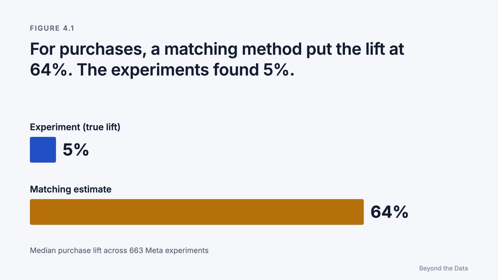
- Across 663 Meta experiments, the median true lift for lower-funnel campaigns was 5%; a machine-learning estimator put it at 24% and a matching estimator at 64% (Gordon et al., 2023). [Experiment vs observational]
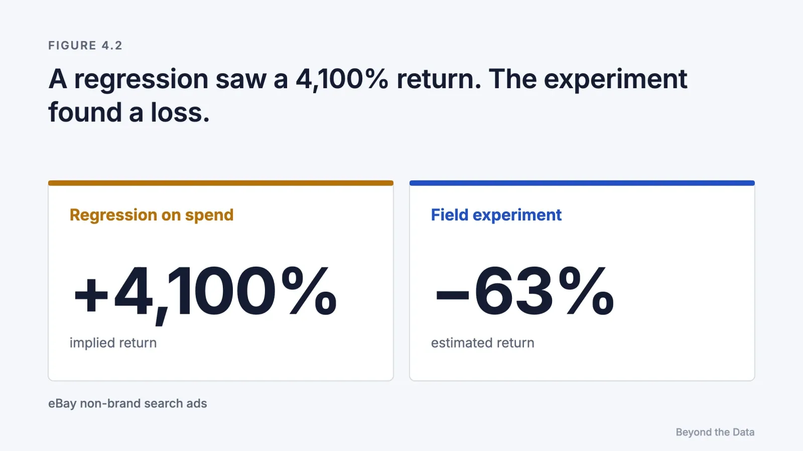
- For eBay's non-brand search ads, a standard regression implied a return of over 4,100%; the experiment found −63% (Blake et al., 2015). [Experiment vs observational]
- Platform A/B tests compare ads shown to different, algorithmically chosen audiences, which can reverse the sign of a result (Braun & Schwartz, 2025). [Analytical]
Short answer. Because the people who see an ad differ from the people who don't in ways that also predict buying. Platforms target likely buyers, active users see more of everything, and algorithms deliver different ads to different audiences. Statistical controls reduce these differences but do not remove them. When the same campaigns were measured both ways, observational methods typically overstated the experimental effect, often several times over.
What is an observational measurement?
An observational measurement estimates the effect of an ad from data in which nobody controlled who saw it. It compares exposed and unexposed people, or periods with more and less advertising, and adjusts for observed differences between them. Attribution models, dashboards, before-and-after comparisons, regressions and most media mix models are observational.
The question is not whether observational methods are useful. They are often the only option. The question is how wrong they tend to be, and in which direction. Advertising offers an unusual opportunity to answer it, because platforms have run thousands of randomised experiments whose true answers can be compared with what observational methods would have estimated from the same data.
How far apart are observational estimates and experiments?
Far enough to change decisions.
Gordon, Zettelmeyer, Bhargava and Chapsky (2019) used 15 US advertising experiments at Facebook, covering 500 million user-experiment observations and 1.6 billion impressions. For each experiment, they applied the observational methods a well-equipped analyst would use, from simple exposed-versus-unexposed comparisons to matching and regression on rich user data, and compared the result with the experiment. In half of the studies, every observational method they tried missed the experimental purchase lift by a factor of three or more. The errors were usually overstatements, sometimes understatements, and no method was reliably better than the others. In one study, the naive comparison of exposed and unexposed users implied a lift of 217%. [Authors declare they received no payment from Facebook]
Gordon, Moakler and Zettelmeyer (2023) repeated the exercise at scale, with 663 experiments.
| Funnel stage of outcome | Experimental median lift | Double machine learning | Stratified propensity score matching |
|---|---|---|---|
| Upper funnel | 29% | 83% | 173% |
| Mid funnel | 18% | 58% | 176% |
| Lower funnel (e.g., purchase) | 5% | 24% | 64% |
Even with rich user-level data and modern machine-learning methods, the authors conclude that the causal effect of a campaign could not be estimated reliably from observational data. [Experiment vs observational; authors include a Meta employee and part-time Meta researchers]
Blake, Nosko and Tadelis (2015) reached the same conclusion for search. For eBay's non-brand keyword ads, a standard regression of sales on search spending suggested a return above 4,100%, still above 1,400% with controls. The field experiment estimated a return of −63% (95% interval −124% to −3%). Most of the ad spending went to frequent eBay users whose purchases did not depend on the ads.
Where does the overstatement come from?
Four mechanisms account for most of it.
| Mechanism | What happens | Evidence |
|---|---|---|
| Targeting selection | Platforms show ads to people already likely to buy, so exposed people would have bought more even without the ad | Lewis & Rao (2015); Blake et al. (2015) |
| Activity bias | People who are very active online on a given day see more ads and also do more of everything, including visiting the advertiser | Lewis, Rao & Reiley (2011) |
| Divergent delivery | In platform A/B tests, each ad version is delivered by the algorithm to a different set of users, so the comparison mixes ad content with audience | Braun & Schwartz (2025) |
| Measurement pressure | When a number becomes a target, the system adapts to move the number, including algorithms that optimise toward attributed conversions | Campbell (1979); Berman (2018) |
The first two biases push estimates upward. Divergent delivery can push them either way, including reversing which ad version looks better. Braun and Schwartz also note that platforms have little incentive to separate the effect of the ad from the effect of the audience, because their optimisation is designed to combine them.
Campbell's law, formulated for social policy, states that the more a quantitative indicator is used for decisions, the more it is exposed to pressures that distort it. Advertising has automated the pressure: bidding algorithms are trained to find the people most likely to produce an attributed conversion, which is not the same as the people most likely to be persuaded.
Why did the number move?
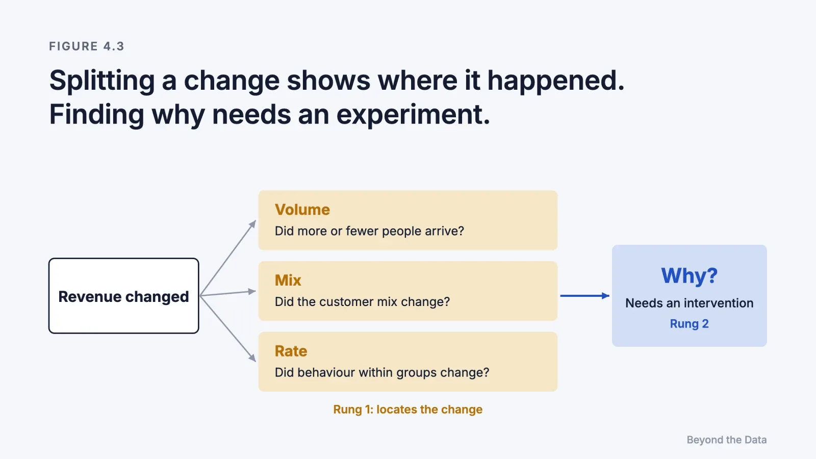
Many measurement questions in practice are not about the size of an effect but about a change: revenue fell 20% last week, or a channel's ROAS halved. Before asking whether advertising caused the change, it helps to locate it. Any change in an aggregate can be split into three parts.
| Component | Question | Example |
|---|---|---|
| Volume | Did more or fewer people arrive? | Traffic fell 15% after a holiday |
| Mix | Did the composition change? | A larger share of new customers, who convert less |
| Rate | Did behaviour within each group change? | Returning customers converted less often |
Illustrative framework.
Mix effects are the classic trap. If a campaign attracts many new visitors, the overall conversion rate can fall even though the conversion rate of every group rose. This is the pattern statisticians call Simpson's paradox (Simpson, 1951): an association that holds within every subgroup reverses when the groups are combined.
A decomposition tells you where the change happened. It does not tell you why. A drop concentrated among returning customers could be caused by an advertising change, a price change, a competitor, or a website problem. Locating a change is rung 1 of the ladder. Explaining it requires rung 2.
There is one useful bridge. When a change was planned, such as a campaign launch in some markets, time-series methods can estimate what would have happened without it by building a synthetic version of the treated market from untreated ones. Brodersen and colleagues (2015) developed a Bayesian structural time-series method for this, released as the CausalImpact package. It is still observational, but it estimates the missing outcome explicitly, which is what Chapter 5 will require.
Can better data or better models fix the problem?
[Our reading] The evidence says: not reliably. The 663-experiment study used far richer data than most advertisers have, and the best observational method still overstated lower-funnel effects nearly fivefold. More data reduces noise. It does not remove selection, because the selection is created by the same targeting that produces the data.
This does not make observational data worthless. It makes it a different kind of evidence: good for describing, ranking and spotting change, weak for sizing causal effects, and least reliable exactly where targeting is strongest, such as retargeting and brand search.
The limit of this chapter
Observational methods can locate a change and describe an association. To know what an ad caused, someone has to decide who sees it, at random, and compare. Chapter 5 describes how.
References
- Berman, R. (2018). Beyond the last touch: Attribution in online advertising. Marketing Science, 37(5), 771–792. doi:10.1287/mksc.2018.1104
- Blake, T., Nosko, C., & Tadelis, S. (2015). Consumer heterogeneity and paid search effectiveness: A large-scale field experiment. Econometrica, 83(1), 155–174. doi:10.3982/ECTA12423
- Braun, M., & Schwartz, E. M. (2025). Where A/B testing goes wrong: How divergent delivery affects what online experiments cannot (and can) tell you about how customers respond to advertising. Journal of Marketing, 89(2), 71–95. doi:10.1177/00222429241275886
- Brodersen, K. H., Gallusser, F., Koehler, J., Remy, N., & Scott, S. L. (2015). Inferring causal impact using Bayesian structural time-series models. Annals of Applied Statistics, 9(1), 247–274. doi:10.1214/14-AOAS788
- Campbell, D. T. (1979). Assessing the impact of planned social change. Evaluation and Program Planning, 2(1), 67–90. Reprinted (2011), Journal of MultiDisciplinary Evaluation, 7(15). doi:10.56645/jmde.v7i15.297
- Gordon, B. R., Zettelmeyer, F., Bhargava, N., & Chapsky, D. (2019). A comparison of approaches to advertising measurement: Evidence from big field experiments at Facebook. Marketing Science, 38(2), 193–225. doi:10.1287/mksc.2018.1135
- Gordon, B. R., Moakler, R., & Zettelmeyer, F. (2023). Close enough? A large-scale exploration of non-experimental approaches to advertising measurement. Marketing Science, 42(4), 768–793. doi:10.1287/mksc.2022.1413
- Lewis, R. A., & Rao, J. M. (2015). The unfavorable economics of measuring the returns to advertising. Quarterly Journal of Economics, 130(4), 1941–1973. doi:10.1093/qje/qjv023
- Lewis, R. A., Rao, J. M., & Reiley, D. H. (2011). Here, there, and everywhere: Correlated online behaviors can lead to overestimates of the effects of advertising. Proceedings of WWW 2011, 157–166. doi:10.1145/1963405.1963431
- Simpson, E. H. (1951). The interpretation of interaction in contingency tables. Journal of the Royal Statistical Society, Series B, 13(2), 238–241.
Chapter 5
How do you measure what an ad caused?
Key findings
- Ghost ads measure lift as precisely as conventional holdout tests at least ten times more cheaply (Johnson, Lewis & Nubbemeyer, 2017). [Experiment]
- In a ghost-ad test of display retargeting for an online retailer, the ads raised website visits by 17.2% and purchases by 10.5% (Johnson et al., 2017). [Experiment]
- A conclusive online advertising experiment can need more than 10 million person-weeks (Lewis & Rao, 2015). [Experiment]
- Synthetic controls are reliable only under specific conditions, including a good pre-period fit and enough comparison units (Abadie, 2021). [Methodological review]
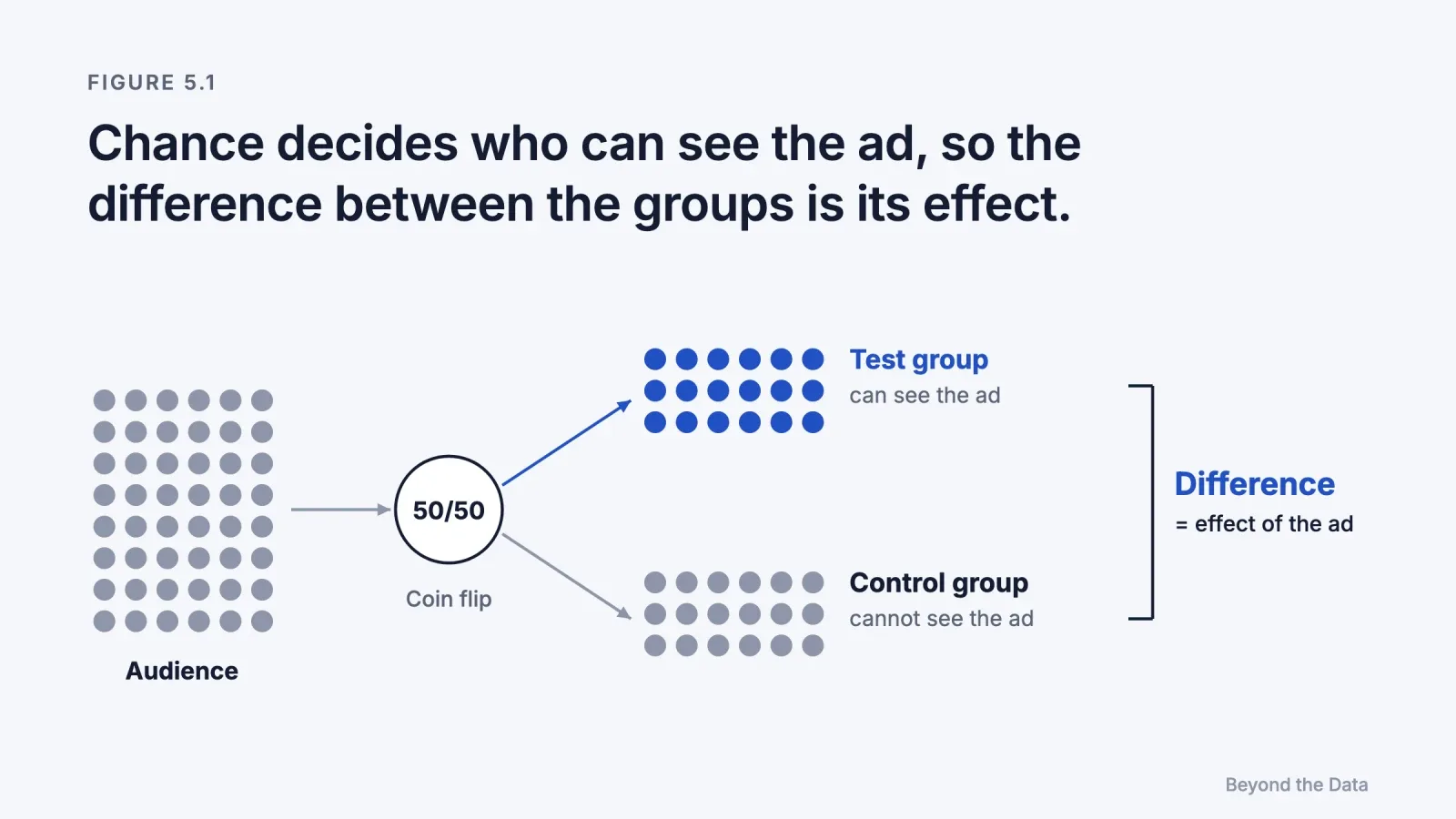
Short answer. Decide at random who can see the ad, then compare outcomes between the groups. Because chance alone decided exposure, the groups are alike in everything except the ad, and the difference estimates its causal effect. User-level holdouts, ghost ads and geographic experiments are the main designs. Each has a cost, a minimum size and a blind spot.
What is an incrementality test?
An incrementality test is an experiment that randomly withholds advertising from part of an audience or some regions and measures the difference in outcomes between the groups. The difference is the incremental effect: the sales that happened because of the ads. Dividing incremental revenue by spend gives incremental return on ad spend (iROAS), the number a budget decision actually needs.
The logic is the one introduced in Chapter 1. The effect of an ad is the gap between two worlds, with and without it. Random assignment creates both worlds at once, in two groups that differ only by chance and by the ad.
Which experimental designs exist?
| Design | Unit randomised | How the control group is formed | Main strength | Main blind spot |
|---|---|---|---|---|
| Intent-to-treat holdout | User | A random share of the target audience is never eligible for the ad | Simple and unbiased | Most people in both groups would never have seen the ad, so the signal is diluted |
| PSA (placebo) ads | User | Control users see an unrelated ad, such as a charity message | Identifies who would have been exposed | The advertiser pays for the placebo impressions; delivery algorithms may treat the two ads differently |
| Ghost ads | User | The platform logs control users who would have seen the ad, without showing anything | Precise and cheap | Requires the platform's cooperation; the advertiser cannot audit the implementation |
| Geo experiment | Region | Advertising is switched off or changed in randomly chosen regions | Measures total store sales, across all channels and offline | Needs many comparable regions; regions are noisy |
| Synthetic control | Region (often few) | A weighted combination of untreated regions imitates the treated one | Works when only one or a few regions can be treated | Not randomised; valid only if the pre-period fit is good |
| Budget-level test | Time or region | Budgets are set at random to different levels | Measures the marginal return, not just on/off | Needs several periods; effects can spill between periods |
Why are ghost ads important?
Because they solve the economics problem described in Chapter 1. In an ordinary holdout, the control group contains everyone in the target audience, including the many who would never have been reached. Their purchases add noise without adding information.
Johnson, Lewis and Nubbemeyer (2017) proposed recording, for each control user, the moment the ad system would have shown the ad, and then comparing only those "would-have-been-exposed" users with actually exposed ones. Their implementation logged more than 100 million predicted ghost ads per day. Compared with intent-to-treat and PSA designs, it measured lift just as precisely at a cost at least an order of magnitude lower. In their application to display retargeting, the ads increased website visits by 17.2% and purchases by 10.5%. [Experiment]
Two lessons follow. First, retargeting can work: this is a positive, experimentally measured effect. Second, it is far smaller than the gaps that naive comparisons of exposed and unexposed users produce, such as the 217% lift in the Facebook study in Chapter 4. The difference is the selection described there.
When should you use a geographic experiment?
When you want to measure total sales rather than tracked conversions, or when the platform cannot run a user-level test. A geo experiment changes advertising in some regions and compares total sales there with regions left untouched. Because it measures store sales from every source, it captures effects that tracking misses: buyers who saw a video and later searched, bought offline, or used another device.
A worked example shows both the power and the trap of geo tests.
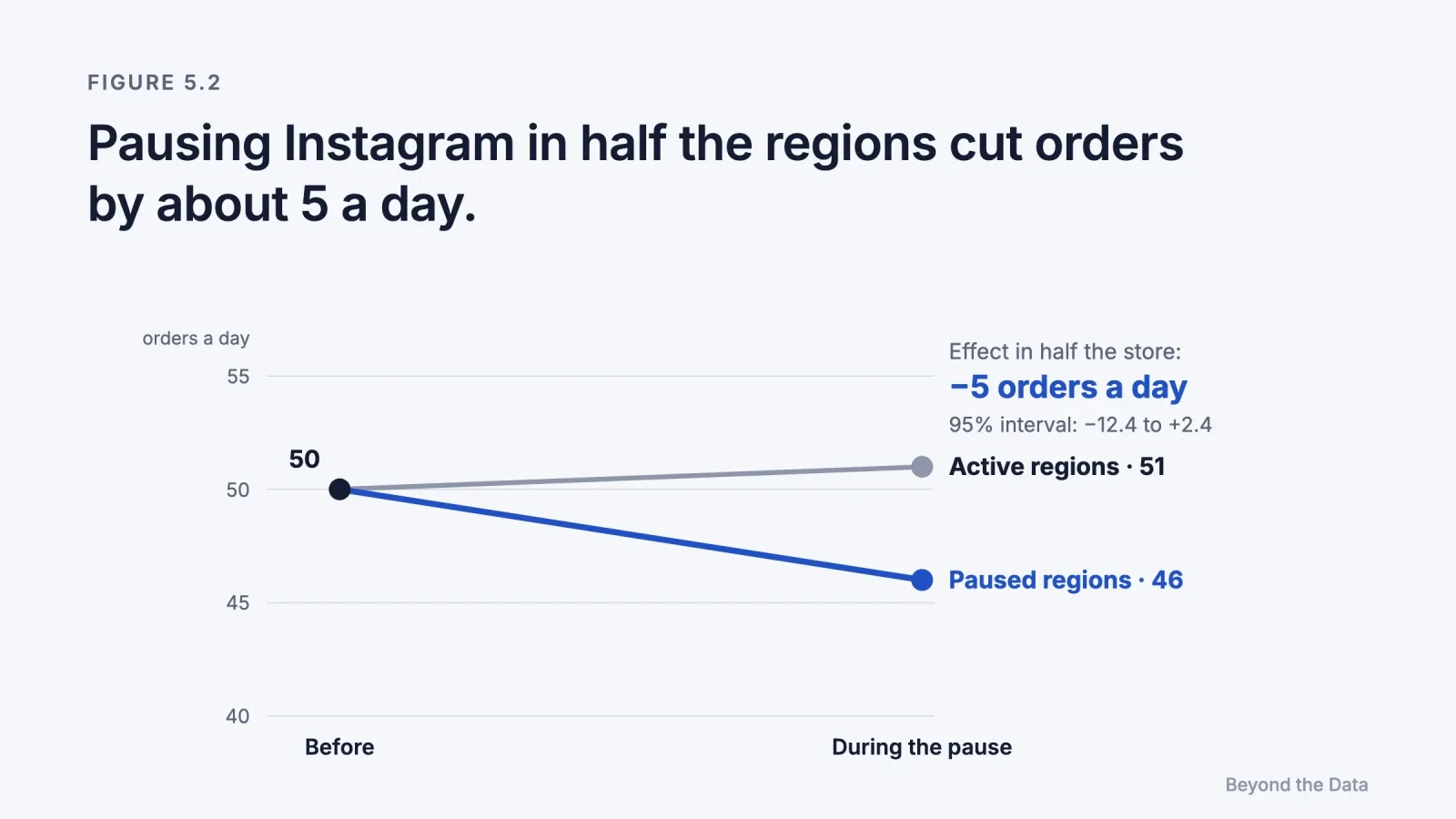
A store pauses Instagram in 4 of its 8 delivery regions, chosen by coin flip, for 14 days. In the 14 days before the pause, both groups averaged 50 orders a day. During the pause, the paused regions averaged 46 and the active regions 51.
- Change in paused regions: 46 − 50 = −4
- Change in active regions: 51 − 50 = +1
- Estimated effect in the paused half: −4 − (+1) = −5 orders a day
- Effect for the whole store (8 regions): about −10 orders a day
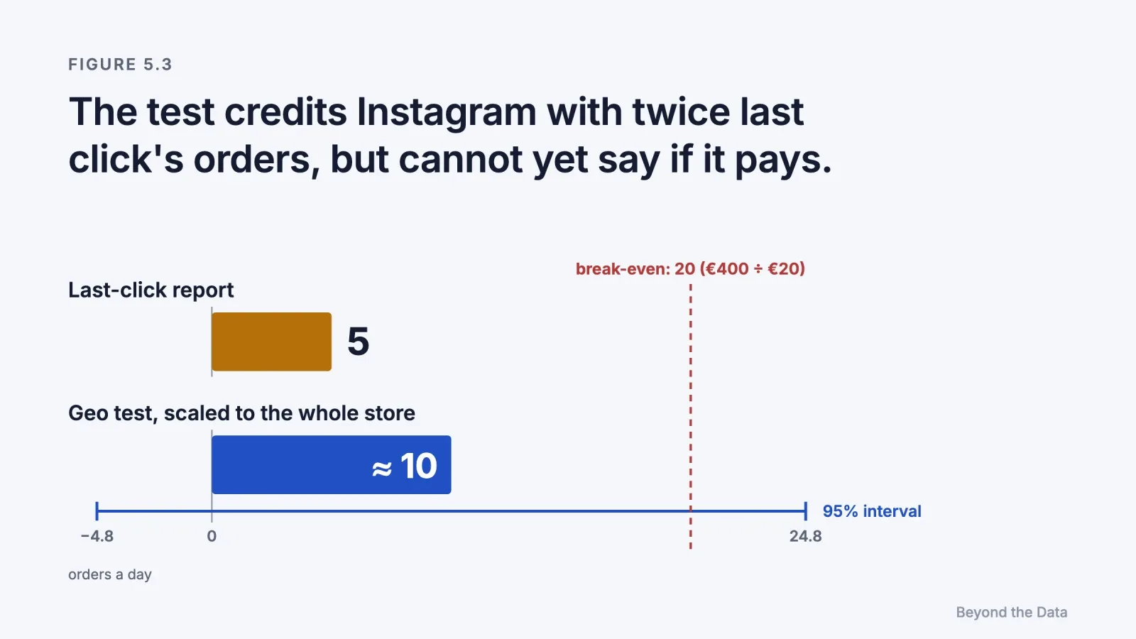
At €20 of profit per order, the central estimate puts Instagram's value at about €200 a day against €400 of daily spend. Last-click reports credit it with 5 orders a day, half of what the test estimates.
Illustrative example. An effect of about 10% of the store's orders is close to the purchase lifts in published experiments: a median of 5% for lower-funnel outcomes across 663 experiments (Chapter 4) and 10.5% for retargeting (above). Case 3 of the test in Chapter 8 uses the same design with a much larger effect.
Two steps are easy to get wrong. The active regions also moved, by +1, so the effect is the difference between the two changes, not the change in the paused regions alone. And the test covered half of the store, so the result has to be scaled to the whole store before it is compared with whole-store spend. Chapter 8 shows that AI analysts skipped the second step in most of their answers.
The estimate also needs an interval. If orders arrive independently of each other, a daily count that averages 50 varies by about √50 ≈ 7 orders, so the daily gap between two such groups varies by about √(50 + 50) = 10. The effect compares the average gap over the 14 days before the pause with the average gap over the 14 days of the pause:
- Standard error of each 14-day average gap: 10 ÷ √14 ≈ 2.7
- Standard error of the effect: √2 × 2.7 ≈ 3.8
- 95% interval in the paused half: −5 ± 1.96 × 3.8 → −12.4 to +2.4 orders a day
- Whole store: −24.8 to +4.8 orders a day, so Instagram's value lies between about −€96 and €496 a day
The interval runs from no effect to just above the €400 of spend. Fourteen days show that last click undercounts Instagram, but they cannot show whether Instagram pays for itself. With 6 weeks before and 6 weeks during the pause, the whole-store interval would narrow to about €30–€370 a day if the central estimate held, below the spend at both ends. Even that interval is optimistic: it assumes that days are independent and that the only noise is the chance arrival of orders, while real regions also differ in weather, delivery and local events. Effects that arrive after the test ends are missed (Chapter 6). The formulas are in Appendix F.
Meta's open-source GeoLift package was built for this design, and Brodersen and colleagues' CausalImpact package supports time-series versions of it.
What makes an experiment trustworthy?
Random assignment removes selection bias but not every error. The literature on online experiments (Kohavi, Tang & Xu, 2020) recommends a short list of checks, which apply directly to advertising tests.
- Decide the metric and the duration before starting. Stopping when the result looks good inflates false positives.
- Check the split. If the groups do not have the sizes the design intended, something in the assignment is broken, and the result should not be trusted.
- Measure total outcomes. Use store revenue or orders, not platform-attributed conversions, which inherit the problems of Chapter 2.
- Allow for delay. Some effects arrive weeks after exposure. A test that stops too early understates them.
- Know who randomised. A platform's lift test is an experiment, but its exposed group is chosen by the platform's delivery algorithm, so comparisons between two ads are subject to the divergent delivery problem (Braun & Schwartz, 2025).
- Report the interval, not only the estimate. With the noise levels in Chapter 1, an honest result often includes both a loss and a large gain.
What can't an experiment tell you?
[Our reading] An experiment answers one question well: what this campaign, in this period, for this audience, caused. It does not answer three others.
- Other budgets. Switching a channel off says what the channel is worth at its current spend. It does not say what the next €1,000 would bring.
- Other times. Effects change with seasons, creative and competition. An experiment from last spring is evidence about last spring.
- Other channels. Testing one channel at a time misses interactions between them, which Chapter 3 showed can be large.
Varian (2016) makes the general case that business decisions require exactly this counterfactual reasoning, and that experiments, where feasible, are the most direct route to it. The practical problem is that a business cannot run an experiment for every channel, at every budget level, every month.
The limit of this chapter
Experiments are local and expensive. A budget decision needs more than an on/off answer for one channel: it needs to know how returns change as spend rises, how long effects take to arrive, and how channels interact. Chapter 6 asks how budget should follow evidence.
References
- Abadie, A. (2021). Using synthetic controls: Feasibility, data requirements, and methodological aspects. Journal of Economic Literature, 59(2), 391–425. doi:10.1257/jel.20191450
- Braun, M., & Schwartz, E. M. (2025). Where A/B testing goes wrong. Journal of Marketing, 89(2), 71–95. doi:10.1177/00222429241275886
- Brodersen, K. H., Gallusser, F., Koehler, J., Remy, N., & Scott, S. L. (2015). Inferring causal impact using Bayesian structural time-series models. Annals of Applied Statistics, 9(1), 247–274. doi:10.1214/14-AOAS788
- Johnson, G. A., Lewis, R. A., & Nubbemeyer, E. I. (2017). Ghost ads: Improving the economics of measuring online ad effectiveness. Journal of Marketing Research, 54(6), 867–884. doi:10.1509/jmr.15.0297
- Kohavi, R., Tang, D., & Xu, Y. (2020). Trustworthy Online Controlled Experiments: A Practical Guide to A/B Testing. Cambridge University Press. doi:10.1017/9781108653985
- Lewis, R. A., & Rao, J. M. (2015). The unfavorable economics of measuring the returns to advertising. Quarterly Journal of Economics, 130(4), 1941–1973. doi:10.1093/qje/qjv023
- Meta. GeoLift: open-source geo experimentation. https://github.com/facebookincubator/GeoLift
- Varian, H. R. (2016). Causal inference in economics and marketing. Proceedings of the National Academy of Sciences, 113(27), 7310–7315. doi:10.1073/pnas.1510479113
Chapter 6
How should budget follow evidence?
Key findings
- For more than 80% of 288 TV-advertising brands, the marginal return was negative, even though the overall return was positive for about a third of them (Shapiro et al., 2021). [Observational]
- Attribution credit is proportional to a medium's marginal effectiveness multiplied by its past exposure; the profit-maximising budget does not depend on past exposure (Danaher & van Heerde, 2018). [Model]
- When two media reinforce each other, the optimal response is to raise total spend and shift some budget toward the less effective medium (Naik & Raman, 2003). [Model, market data]
- In media mix models, the estimated optimal mix can vary widely because the underlying parameters are uncertain (Jin et al., 2017). [Model]
Short answer. Budget should follow the marginal return: what the next euro in a channel adds to total profit. Average return on ad spend, the number most reports show, describes the euros already spent. Saturation makes the margin lower than the average, delayed effects make short windows understate it, and synergy means a channel's margin depends on the others. When the evidence is weak, the best decision is often to keep the current budget and test.
What is the difference between average and marginal return?
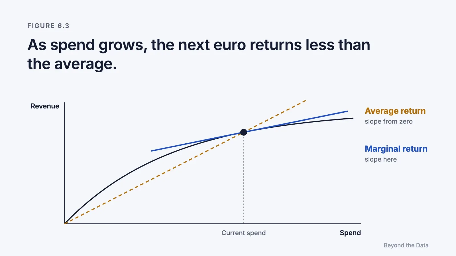
The average return on ad spend divides all the revenue credited to a channel by all the money spent on it. The marginal return is the extra profit from the next unit of spend. Budget decisions are always about the next unit: whether to add, cut or move money. The average is therefore the wrong number for the decision, even when it is measured correctly.
An experiment from the test in Chapter 8 shows how far the two can diverge.
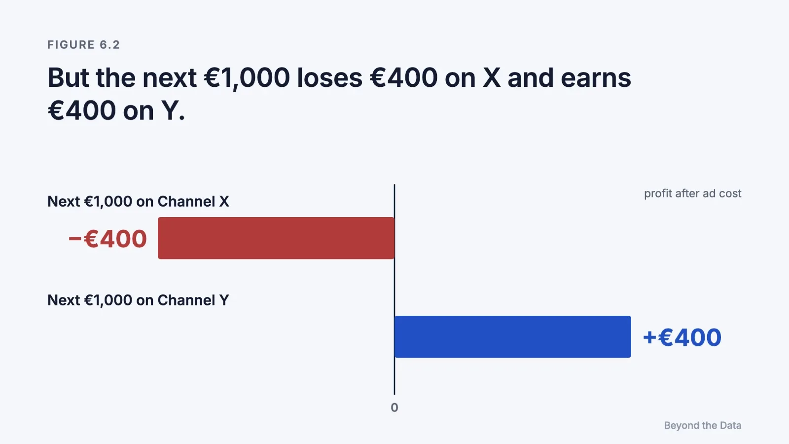
Over 8 weeks, a store set the weekly budgets of Channel X and Channel Y at random, each to either €2,000 or €3,000. Average weekly store revenue:
| Weeks where | Revenue |
|---|---|
| X at €2,000 | €40,100 |
| X at €3,000 | €41,300 |
| Y at €2,000 | €39,300 |
| Y at €3,000 | €42,100 |
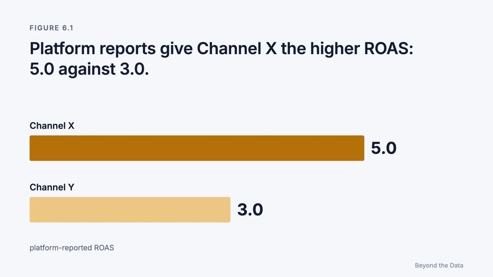
Platform-reported ROAS: X 5.0, Y 3.0. Half of revenue is profit before ad costs.
- Extra €1,000 on X: +€1,200 revenue → +€600 profit → €400 loss after the spend
- Extra €1,000 on Y: +€2,800 revenue → +€1,400 profit → €400 gain
Illustrative example.
The channel with the higher average return is the worse place for the next euro. This is the normal situation for a channel that has been scaled up: its best audiences were reached first, so its average stays high while its margin falls.
How sure is that ranking? Suppose each of the four budget combinations fell in 2 of the 8 weeks, and weekly revenue varies around its expected level with a standard deviation of €500. Each channel's effect then compares 4 weeks with 4 weeks:
- Standard error of each channel's effect: €500 × √(1/4 + 1/4) ≈ €354, so the 95% interval is about ±€690
- X: +€1,200 of revenue (€510 to €1,890) → between about −€750 and −€50 after the extra spend
- Y: +€2,800 of revenue (€2,110 to €3,490) → between about +€50 and +€750 after the extra spend
- Y minus X: +€1,600 of revenue, standard error €500 → €620 to €2,580
With only 8 weeks of data, an interval based on the t-distribution, which multiplies by 2.57 instead of 1.96, is about 30% wider. Y's own gain could then fall slightly below zero, while Y still beats X. The ranking is more certain than the profit. The €500 is an illustrative assumption; Case 2 of the test gives only the averages.
Why does the margin fall as spend rises?
Because of saturation. The first euros in a channel reach the most responsive audiences at the lowest cost. Additional euros reach people who are less interested, more expensive to reach, or already reached. Media mix models capture this with a shape (diminishing-returns) curve (Jin et al., 2017).
Shapiro and colleagues' results on 288 brands show how much it matters. For most brands, the last dollar of TV advertising returned less than it cost, even though the advertising as a whole was profitable for about a third of them (Shapiro et al., 2021). [Our reading] Even in the third of brands where advertising paid overall, an advertiser reading only the average return would conclude that the channel works and would keep scaling it past the point where it pays.
How do delayed effects distort the picture?
Advertising often works with a delay. Someone sees a video today and buys in three weeks. Attribution windows of 1 or 7 days miss this, so channels whose effects arrive late look weaker than they are. Media mix models represent the delay as carryover, or adstock, a decaying effect that continues after the spend (Jin et al., 2017).
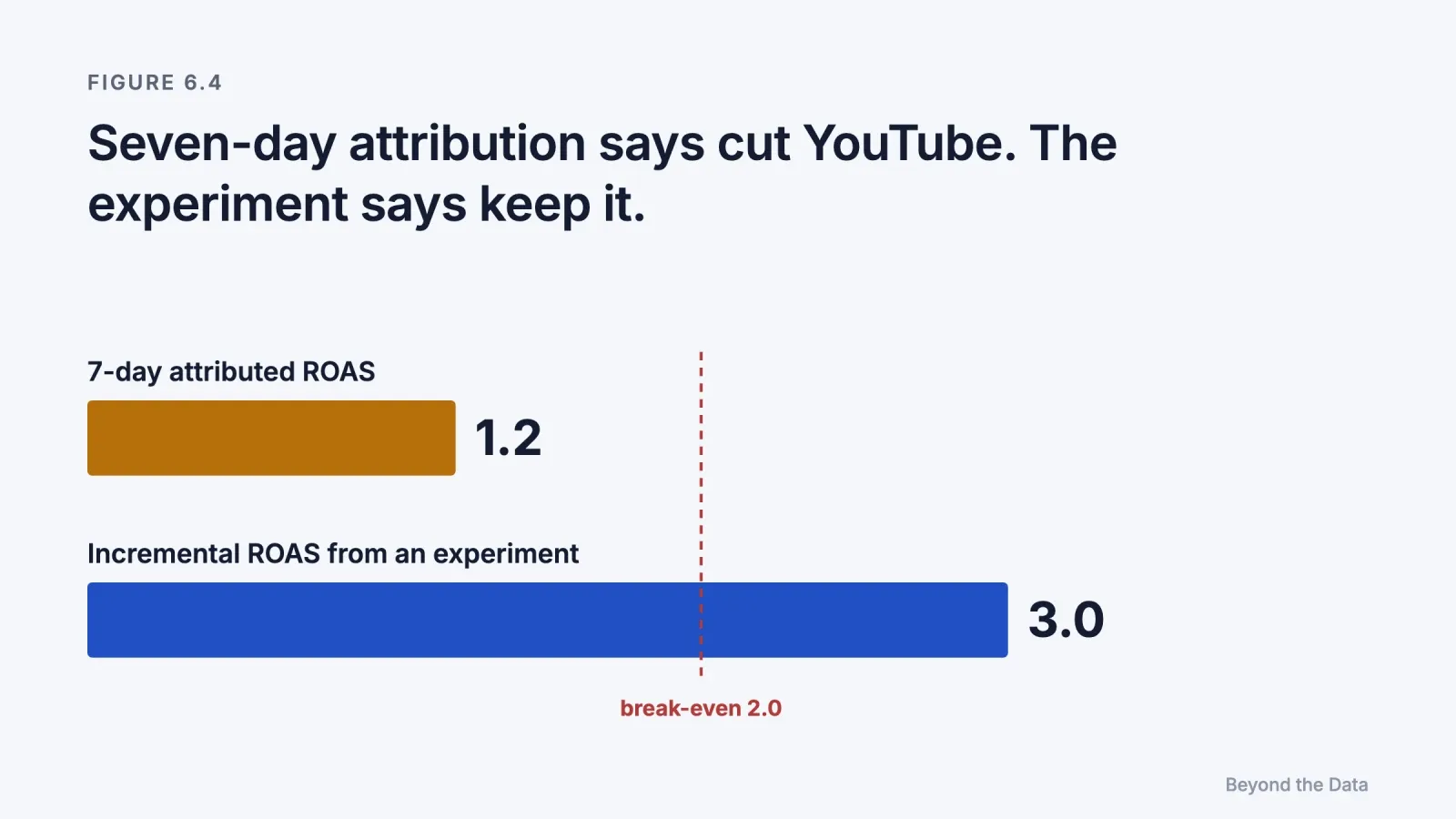
A store spends €5,000 a month on YouTube. The agency dashboard, with 7-day click attribution, shows €6,000 of revenue (ROAS 1.2). Half of revenue is profit, so break-even ROAS is 2.0. A regional experiment last spring estimated €15,000 of incremental revenue per €5,000 of spend (95% interval €10,500 to €19,500), mostly arriving 2 to 5 weeks after exposure.
- Attributed ROAS: 1.2, below break-even → "cut it"
- Incremental ROAS: 3.0, above break-even → about €2,500 a month of profit after ad costs
- Low end of the interval: ROAS 2.1, still above break-even → about €250 a month
Illustrative example used in the test in Chapter 8. The interval is added here; Case 5 of the test gives only the estimate.
The same campaign looks unprofitable or profitable depending on whether the measurement window covers the delay.
How does synergy change the decision?
If channels reinforce each other, as Chapter 3 showed for display and search, a channel's margin depends on how much is spent on the others. Naik and Raman (2003) estimated synergy between TV and print in Dockers' advertising and derived a counterintuitive rule: as synergy rises, an advertiser should spend more in total and shift some budget toward the less effective medium, because that medium increases the return on the more effective one. [Model, market data]
Attribution cannot capture this rule. It assigns each channel a fixed share, while the true value of each channel changes with the others' budgets. Danaher and van Heerde (2018) make a related point in a paper titled "Delusion in Attribution": attribution credit reflects a medium's marginal effectiveness multiplied by its past exposure, while the profit-maximising allocation does not depend on past exposure at all. Allocating by attribution shares therefore tends to reproduce last year's plan.
What should you do when the evidence is uncertain?
Treat the decision as a choice under uncertainty, and price the uncertainty. [Our reading]
| Situation | Evidence available | Typical correct decision |
|---|---|---|
| A trusted experiment shows the channel is profitable, even at the low end of its interval | Experiment, interval above break-even | Keep, whatever attribution says |
| Attribution and an experiment disagree | Experiment and attribution | Follow the experiment, then check whether the attribution window misses delayed effects |
| Two channels compete for one budget increase and a budget-level test exists | Marginal returns from a test | Give the money to the higher marginal return, not the higher average |
| Only attribution exists and platform claims overlap | Attribution only | Keep the budget unchanged and run a test before cutting or scaling |
| Exposed users convert much more than unexposed ones | Observational comparison only | Do not scale on that gap; run a holdout first |
The last two rows deserve emphasis. When the only evidence is attribution, switching a channel off can destroy value that the reports never showed, and scaling a channel can pour money into selection. A short test is usually cheaper than either mistake. The value of a test is the expected loss from the decision it prevents.
An example from Chapter 8's test illustrates the first row.
Google Ads reports 300 conversions on €9,000 of spend; each order brings €45 of profit. A randomised lift test on the same campaigns found that 92% of reported conversions were caused by the ads (95% interval 80–104%).
- Central estimate: 276 incremental orders × €45 = €12,420 profit → about €3,420 above spend
- Low end: 240 orders × €45 = €10,800 → still about €1,800 above spend
A consultant's general claim that "Google takes credit for sales that would have happened anyway" is true in many settings and false here.
Discounting every platform number by a fixed amount is as much of a shortcut as trusting every platform number. The evidence on each channel decides.
The limit of this chapter
Every rule in this chapter needs a response curve for each channel: how returns change with spend, how long they take to arrive, and how they depend on other channels. Experiments supply a few points on those curves. To estimate the whole set together, an advertiser needs a model of all channels at once, and a way to keep it honest. Chapter 7 describes how attribution, experiments and models fit together.
References
- Danaher, P. J., & van Heerde, H. J. (2018). Delusion in attribution: Caveats in using attribution for multimedia budget allocation. Journal of Marketing Research, 55(5), 667–685. doi:10.1177/0022243718802845
- Jin, Y., Wang, Y., Sun, Y., Chan, D., & Koehler, J. (2017). Bayesian methods for media mix modeling with carryover and shape effects. Google Inc.
- Naik, P. A., & Raman, K. (2003). Understanding the impact of synergy in multimedia communications. Journal of Marketing Research, 40(4), 375–388. doi:10.1509/jmkr.40.4.375.19385
- Shapiro, B. T., Hitsch, G. J., & Tuchman, A. E. (2021). TV advertising effectiveness and profitability: Generalizable results from 288 brands. Econometrica, 89(4), 1855–1879. doi:10.3982/ECTA17674
Chapter 7
How do attribution, experiments and models fit together?
Key findings
- Calibrating attribution on 2,226 experiments raised its explanatory power for incremental effects from 19% to 88% (Gordon et al., 2026). [Experiment]
- Bayesian media mix models can represent delayed and diminishing effects, but with small samples the prior assumptions largely determine the result (Jin et al., 2017). [Model]
- Google released Meridian, an open-source Bayesian media mix model, to all advertisers in January 2025 (Google, 2025). [Platform]
- 85% of marketers say they are confident in measuring holistic return on investment, but only 32% actually measure it holistically (Nielsen, 2025). [Industry survey]
Short answer. Each method answers a different question at a different speed. Attribution is fast and biased, so it gives daily direction within channels. Experiments are slow and local, so they give ground truth for a few channels at a time. Media mix models are broad and assumption-heavy, so they spread the evidence across all channels and budgets. Calibration ties them together: experiments correct the model and the attribution, and the model decides where the next experiment is most needed.
What is a media mix model?
A media mix model (MMM) is a statistical model that explains total sales over time with the spend in each advertising channel, plus non-advertising factors such as price, seasonality and promotions. It uses aggregate data, such as weekly sales and weekly spend by channel, so it needs no user-level tracking and is unaffected by the consent and attribution-window problems of Chapter 2.
Modern MMMs include the two features Chapter 6 showed to matter. A carryover term spreads each week's advertising effect over later weeks. A shape term makes returns diminish as spend rises. From these curves the model can compute both the average and the marginal return of each channel (Jin et al., 2017).
What are the limits of a media mix model?
They are serious, and the model's developers state them clearly.
| Limit | Why it matters | Source |
|---|---|---|
| Few data points | Two years of weekly data give about 100 observations to estimate many parameters | Jin et al. (2017); Chan & Perry (2017) |
| Prior dependence | With small samples, the Bayesian prior strongly shapes the estimates and can bias them | Jin et al. (2017) |
| Unstable optimum | In a case study, the recommended media mix varied considerably because parameters were uncertain | Jin et al. (2017) |
| Correlated spend | Channels that are usually increased together cannot be separated by the data | [Our reading] |
| Observational at heart | MMM is still a regression on non-random variation, so it inherits the selection problems of Chapter 4 | [Our reading] |
Chan and Perry (2017), also from Google, describe the difficulties MMMs face in giving consistently reliable answers about media effectiveness. The honest summary is that an MMM is a structured way of combining assumptions with data. Its value depends on how good the assumptions are and how well they are checked.
What does calibration mean?
Calibration means using experimental results to correct a non-experimental measure. It runs in two directions.
- Calibrating the model. An experiment on a channel provides a reliable estimate of its effect at current spend. That estimate is used as an informative prior or a constraint in the MMM, so the model's curve must pass near the experimental point.
- Calibrating attribution. The ratio between experimental and attributed conversions for a channel becomes a correction factor for its daily attribution numbers.
The PIE study is the strongest evidence that calibration works. Using 2,226 Meta experiments, Gordon, Moakler and Zettelmeyer (2026) built a model that predicts a campaign's incremental effect from features that are available without an experiment. Its out-of-sample R² was 0.88, against 0.19 for 7-day last click. [Experiment; one author is a Meta employee]
Platforms have moved in the same direction. Meta's incremental attribution, introduced in 2025, is a model-based estimate of caused conversions. Meta reports that it delivers 24% more incremental conversions than standard attribution, which is a platform statement about its own product (Meta, 2026). Google made Meridian, an open-source Bayesian MMM, available to everyone in January 2025 (Google, 2025), and Meta maintains an open-source MMM called Robyn.
How should the three methods work together?
| Method | Question it answers | Speed | Typical bias | Role in the system |
|---|---|---|---|---|
| Attribution | Which ads and keywords are associated with conversions within a channel? | Daily | Overstates targeted, late-funnel ads; misses untracked buyers | Direction: day-to-day optimisation within a channel |
| Experiments | What did this channel cause, at this spend, in this period? | Weeks | Local in time, budget and audience | Truth: anchor points for everything else |
| Media mix model | How do all channels, budgets and delays combine? | Monthly or quarterly | Depends on assumptions and priors | Allocation: budget across channels |
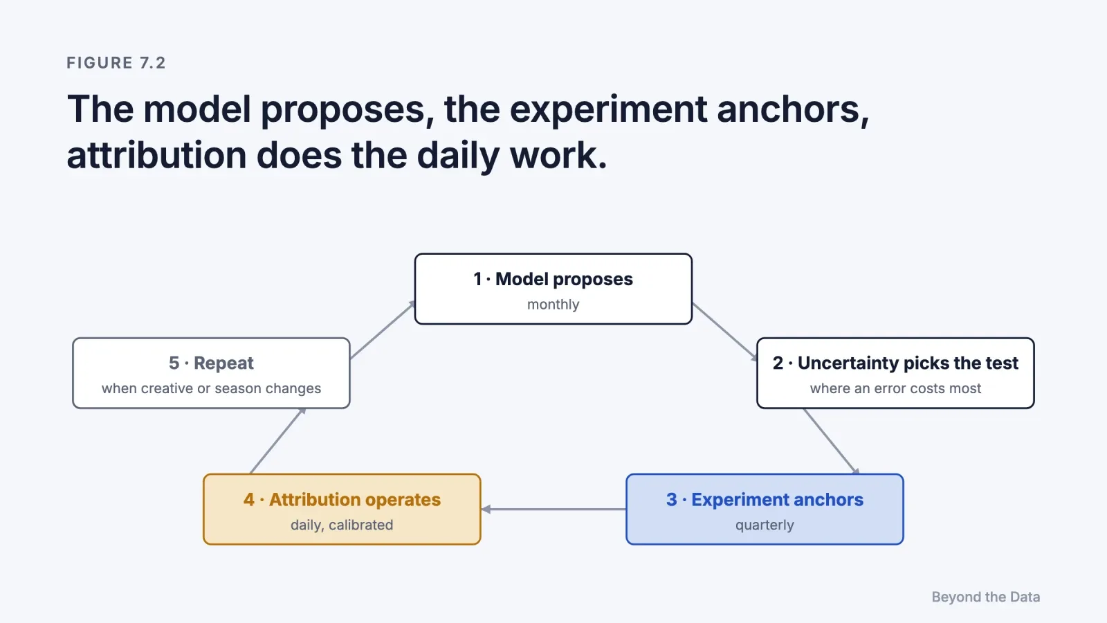
The system works as a loop. [Our reading]
- Model proposes. The MMM estimates each channel's marginal return and its uncertainty.
- Uncertainty chooses the next test. The channel whose estimate is both large and uncertain is tested first, because that is where an error costs the most.
- Experiment anchors. The result updates the MMM and produces a correction factor for that channel's attribution.
- Attribution operates. Teams optimise daily inside channels using calibrated attribution.
- Repeat. Experiments are renewed when campaigns, seasons or creative change.
What does this look like in an operating rhythm?
| Cadence | Activity | Evidence rung |
|---|---|---|
| Daily | Optimise campaigns with calibrated attribution; watch for anomalies | 1 |
| Weekly | Reconcile platform claims with store revenue (Chapter 2) | 0 |
| Monthly | Review MMM marginal returns; adjust budgets within tested ranges | 3 |
| Quarterly | Run one or two experiments where the model is least certain; recalibrate | 2 |
| Yearly | Re-estimate the MMM; review definitions and windows | 0–3 |
The Nielsen figures quoted above suggest how rare this is. Most marketers believe they measure holistically, and about a third do (Nielsen, 2025). [Industry survey]
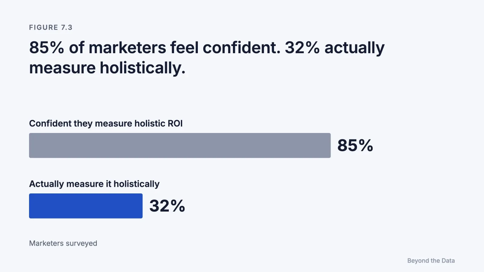
What if a business cannot afford all three?
[Our reading] The system scales down. A small advertiser can run one geo test a quarter on its largest channel, use the result to correct attribution for that channel, and treat every uncorrected channel's attribution as an upper bound rather than an estimate. Even this minimal version moves the reporting stack from rung 1 to rung 2 for the channel that matters most.
The limit of this chapter
The system described here produces more evidence than any team can read in full: thousands of campaign rows, experiment results, model curves and corrections. Increasingly, the reader is an AI assistant asked to summarise the evidence and recommend what to do. Chapter 8 asks whether an AI analyst can tell credit from cause.
References
- Chan, D., & Perry, M. (2017). Challenges and opportunities in media mix modeling. Google Inc.
- Google. (2025, January 29). Meridian is now available to everyone. Google Blog. [Platform]
- Gordon, B. R., Moakler, R., & Zettelmeyer, F. (2026). Predicted incrementality by experimentation (PIE) for ad measurement. arXiv:2304.06828v2.
- Jin, Y., Wang, Y., Sun, Y., Chan, D., & Koehler, J. (2017). Bayesian methods for media mix modeling with carryover and shape effects. Google Inc.
- Meta. (2026, January 28). Fourth quarter 2025 earnings conference call transcript. [Platform]
- Meta. Robyn: open-source marketing mix modeling. https://github.com/facebookexperimental/Robyn
- Nielsen. (2025). 2025 Annual Marketing Report. [Industry survey]
Chapter 8
Can an AI analyst tell credit from cause?
Key findings
- On a benchmark built from real requests on an advertising platform, the best model produced the correct reported answer 76.9% of the time, and 61.4% on the hardest level (AD-Bench, 2026). [Benchmark]
- On pure correlation-to-causation reasoning, most of 17 language models performed close to chance (Jin et al., 2023). [Benchmark]
- In our six-case test, models chose the correct decision in 47.5 of 48 cue-free attempts. [Our test, 48 attempts]
- In 5 of 8 cue-free answers to a geo-test case, the model compared half-store losses with whole-store spend. [Our test]
- In a replication with 120 Claude Haiku 5.5 runs and two independent raters, the model chose the correct decision 703 of 720 times; every miss was in case 1. [Our replication, 120 attempts]
Short answer. In our test, mostly yes, when the evidence is in front of it. Given six advertising cases with known correct answers, two families of language models reached the right decision in 47.5 of 48 cue-free attempts, and pushed back unprompted on proposals that confused credit with cause. Their characteristic failure was arithmetic scale: in five of the first eight answers, a test that covered half of a store was compared with the whole store's spend; in a 120-run replication the same slip appeared in 35 answers. In the original runs, some answers also described interval-based evidence as proof; in the replication none did.
Why does this question matter now?
Because AI assistants have become readers of advertising data. Marketers paste dashboards into chat assistants, and analytics products connect assistants directly to ad accounts. The assistant is asked the question this book is about: what did the advertising cause, and what should we do?
An assistant can fail in two ways. It can repeat the report's credit as if it were cause, which would automate the errors of Chapters 2 to 4. Or it can distrust every number, which would discard good evidence such as experiments. A useful analyst has to do what this book describes: place each piece of evidence on the right rung of the ladder and decide accordingly.
What does existing research say?
| Study | What it measures | Relevance |
|---|---|---|
| AD-Bench (2026) | LLM agents answering real analytical requests on an advertising platform | Best model 76.9% Pass@1, 61.4% on the hardest level. Correct means the reported number, not a causally valid conclusion |
| Jin et al. (2023), CORR2CAUSE | Inferring causal relations from sets of correlational statements, 200,000+ examples, 17 models | Most models close to chance; fine-tuning did not generalise to perturbed queries |
| Kıcıman et al. (2023) | Causal reasoning tasks with GPT-3.5 and GPT-4 | 97% on pairwise causal discovery, 92% on counterfactual reasoning, 86% on event causality, with unpredictable failures; models reason from text, not from the data |
The two causal studies point in opposite directions, and the difference is instructive. Language models do well when causal knowledge is expressed in words they have learned, and poorly when they must derive causation formally from correlations. Advertising analysis needs both.
In a structured search of 225 arXiv records and several journal and industry sources, we found no study that tests whether an AI analyst's conclusions from advertising data are causally valid in scenarios where the true effect is known. AD-Bench comes closest but scores the reported number. This chapter reports a first test of that question.
How did we test it?
We wrote six cases, each a short description of one online store's data and a proposal from the owner, an agency or a consultant. Each case contains one of the traps from this book, and each has a correct decision that follows from the data.
| Case | Trap | Chapter | Correct decision |
|---|---|---|---|
| 1 | Platforms' claims sum to more than store revenue; owner wants to move budget by platform ROAS | 2 | Do not move it yet; test incrementality first |
| 2 | Higher average ROAS, lower marginal return in a randomised budget test | 6 | Give the extra budget to the channel with the higher marginal return |
| 3 | Last click credits Instagram with 5 orders; a randomised regional pause shows it drives about 50 a day, partly through search | 3, 5 | Keep Instagram |
| 4 | Control case: a lift test confirms most of Google's reported conversions; a consultant says "switch it off" | 6 | Keep Google Ads |
| 5 | Attributed ROAS below break-even; an experiment shows delayed effects above it | 6 | Keep YouTube |
| 6 | Retargeted visitors convert at 4×; agency wants to double the budget | 4, 5 | Do not scale; run a holdout first |
The cases are balanced so that two common shortcuts both fail. A model that trusts platform numbers fails cases 1, 3, 5 and 6. A model that discounts every platform number fails cases 4 and 5.
Case 3 gives Instagram a deliberately large effect: about half of the store's orders. Published experiments find much smaller effects, and Chapter 5 works through the same design with a realistic one, where a 14-day test cannot settle the decision. The case tests the two steps of the arithmetic, not the size of the effect.
We ran three versions of the prompt:
- v1: multiple-choice options with computed values;
- v2: a fixed list of decisions, plus a "data enough to decide?" field;
- v3: no options and no fields. The model writes two or three sentences to the owner.
Version 3 removes every cue that hints at testing or at the existence of a "wait" option. It is the version reported below. The models were Claude Haiku 5.5 (three independent runs per version, no tools, no access to the answer key) and Google Gemini (five runs of v3, each in a new chat, through the consumer app as served in November 2026). Answers were scored against the key by the author.
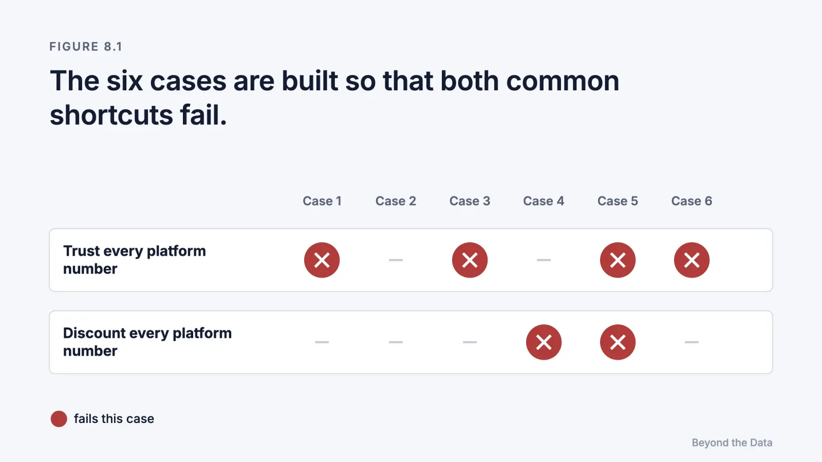
What did the models do?
| Version | Model | Runs | Correct decisions |
|---|---|---|---|
| v1 (options) | Claude Haiku 5.5 | 3 | 18 of 18 |
| v2 (decision list) | Claude Haiku 5.5 | 3 | 18 of 18 |
| v3 (free text) | Claude Haiku 5.5 | 3 | 18 of 18 |
| v3 (free text) | Gemini | 5 | 29.5 of 30 |
| v3 (free text), replication | Claude Haiku 5.5 | 120 | 703 of 720 |
Finding 1: when the evidence is visible, the direction is right. In every cue-free run, both models refused to move budget on overlapping platform claims (case 1) and refused to scale retargeting on the 4× gap (case 6). They recommended a holdout or geo test without being prompted to. They kept Google Ads against the consultant's general claim (case 4) and used the experiment, not the 7-day attribution, for YouTube (case 5). Removing the cues did not change the scores, which suggests that the cases display their evidence too plainly to separate the models. [Our reading] A larger Haiku replication, reported below, found that case 1 is not solved in every run.
Finding 2: the arithmetic scale breaks. Case 3 requires two steps described in Chapter 5: subtract the change in the control regions, and scale the half-store result to the whole store.
| What the answer computed | Answers (of 8) |
|---|---|
| Whole-store loss, control-adjusted (about €1,000 a day) | 1 |
| Whole-store loss, not control-adjusted (€960) | 1 |
| Half-store loss only (€480–500), compared with whole-store spend (€400) | 5 |
| No calculation | 1 |
The decision was still correct, because €480–500 exceeds €400. At €600 of daily spend, the same comparison would point the wrong way. In the Haiku replication below, 35 of 120 answers made this comparison at €400; when we raised the spend to €600, only 6 of 120 did, and none switched Instagram off.
Finding 3: one causal misreading. One Gemini answer treated the fall in search clicks in the paused regions as a confounder that made Instagram's effect "difficult to isolate", and asked for another experiment. The fall in search clicks is part of Instagram's effect, the complementarity of Chapter 3. This was the only answer scored as a half point.
Finding 4: overconfident language. Several answers said that an experiment "proves" an effect, including for a lift estimate whose interval ran from 80% to 104%. Chapter 1 showed why advertising experiments rarely prove anything precisely. One answer instead reported the full interval and showed that the decision held even at its low end. In the Haiku replication below, no answer called the evidence proof.

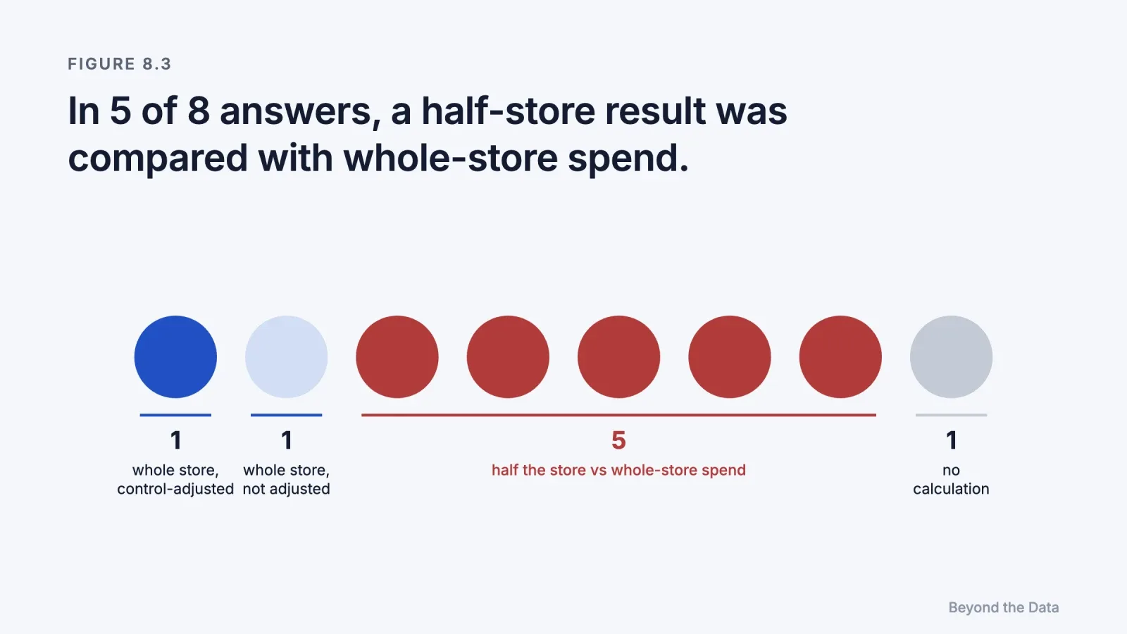
Did the result hold in a larger run?
We repeated version 3 with Claude Haiku 5.5 on 18 November 2026: 120 independent runs, a scoring rubric fixed before any answer was generated, and two independent model raters (Claude Haiku 5.5 and Claude Sonnet 5.5) who did not see each other's scores. Disagreements were resolved by reading each answer. The runs used an agent environment rather than a plain chat, and the Haiku version was fixed only by the date of the run. [Our replication]
| Case | Correct decisions (of 120) |
|---|---|
| 1 | 103 |
| 2–6 | 120 each |
| Total | 703 of 720 |
Three results differ from the eight original runs.
- Case 1 is not solved every time. Case 1 was identical in both Haiku runs reported here, 240 answers including the €600 run below. In 22 of the 240, the model saw that platform claims exceed store revenue, then advised shifting or cutting part of the budget now, mostly while watching store revenue: a before-and-after comparison without a control. Depending on how strictly a shift presented as a test is read, the count is 16 to 22. At a failure rate near 9%, three clean runs out of three happen about three times in four, so the original 18 of 18 is consistent with this result.
- The half-store slip is common but not the majority. Of 120 answers, 41 scaled and adjusted correctly, 26 scaled without the control adjustment, 35 compared half-store loss with whole-store spend, and 18 took another route, most of them comparing half-store loss with half-store spend (€200), which is also correct. Of the 35, about eight stated the comparison as a deliberate lower bound ("in half the store alone"), and six concluded that Instagram's margin was thin, when the scaled result is about €1,000 of profit against €400 of spend.
- No Haiku answer called the evidence proof. Answers that used the word said "not proof". In case 4, 116 of 120 answers also checked the decision at the 80% low end of the lift interval.
What if the slip would change the decision? We then ran 120 more Haiku answers with one change to the prompt: Instagram's daily spend in case 3 rose from €400 to €600, so that comparing half-store loss with whole-store spend would point toward switching Instagram off. The rubric and the two raters were the same; a decision code and one more arithmetic code were added before the run. Only 6 of 120 answers made the half-store comparison, against 35 of 120 at €400. Of the 120 answers, 115 kept Instagram, 2 advised reducing it, 3 asked for another test before deciding, and none switched it off. Both answers that advised reducing it were among the six that made the slip. Gemini was not retested at €600. [Our replication]
The original eight answers mixed two model families, so the replication shows Haiku's rates; it does not correct Gemini's. The raters were language models, not a second person. Their raw agreement was 97–100% on decisions and 78% on the case 3 arithmetic code.
What does the test show, and what does it not show?
[Our reading] It shows that current models, given clean cases with visible evidence, apply the main distinctions of this book: platform claims versus store totals, average versus marginal return, attributed versus incremental effect, and correlation from targeting versus causation. It shows that their weak point is quantitative transfer, the step from "what the test measured" to "what it means for this business".
It does not show how models perform on real reports, where the decisive fact is buried among dozens of rows, several traps occur together, and nothing says which number matters. Our cases put the decisive evidence in a few sentences. The results are therefore an upper bound.
Limitations. The test has six cases written by the author, two model families, eight runs of version 3, and scoring of the original runs by one person; the Haiku replication used two model raters but no second human. ChatGPT was planned but not tested. The consumer version of Gemini was not pinned to a specific model version. The author's company builds analytics tools that use AI assistants, which is a reason to read the results with care, and the reason the full prompts and answer key are published in Appendix D.
The next step is a harder test: realistic multi-channel reports with the evidence embedded, combined traps, and the €600 version of the half-store trap run on other model families.
How should you use an AI analyst on advertising data?
[Our reading] Six instructions turn the findings into practice.
- Give it the store total. Without it, the model cannot detect overlapping platform claims.
- Ask for the rung. For every claim, ask whether it comes from a platform report, an attribution model, an experiment or a model.
- Ask for the missing world. Ask what would have happened without the ads, and how the answer knows.
- Check the scale. When a test covered part of the audience or some regions, check that the result was scaled before being compared with total spend.
- Ask for the interval. A decision that only holds at the central estimate is a weaker decision than one that holds across the interval.
- Treat "proves" as a warning. Advertising evidence is rarely proof. An analyst who says it is has skipped a step.
The limit of this chapter
An AI analyst can climb the ladder only as high as the evidence it is given. If the reporting stack contains only attribution, the best analyst can only say so and recommend a test. The ladder, not the reader, sets the ceiling. The Conclusion collects the book's argument into twelve propositions.
References
- Hu, L., Sun, Y., Xia, T., Li, W., Xu, M., Xu, L., Wang, S., Xu, W., Jiang, J., et al. (2026). AD-Bench: A real-world, trajectory-aware advertising analytics benchmark for LLM agents. arXiv:2602.14257.
- Jin, Z., Liu, J., Lyu, Z., Poff, S., Sachan, M., Mihalcea, R., Diab, M., & Schölkopf, B. (2023). Can large language models infer causation from correlation? arXiv:2306.05836.
- Kıcıman, E., Ness, R., Sharma, A., & Tan, C. (2023). Causal reasoning and large language models: Opening a new frontier for causality. arXiv:2305.00050.
Conclusion
Twelve propositions
Each proposition stands on its own and names the chapter where its evidence is set out.

1. The effect of an ad is a difference between two worlds, and a report shows only one of them. Credit is the share of a sale a report assigns to an ad. Cause is the share that would disappear without it. Every measurement method is a way of estimating the missing world, or of not trying. (Chapter 1)
2. Advertising effects are small compared with the noise in sales. Typical elasticities are around 0.1 to 0.2, and confidence intervals for the return on a single campaign are often more than 100 percentage points wide. A very large reported return is more likely to reflect selection than effect. (Chapter 1)
3. A reported conversion is a claim made under a definition. The event, the link to a person and the time window are all choices. When a platform changes them, the number changes although no customer did. (Chapter 2)
4. When platform claims add up to more than the store's revenue, their return figures cannot be compared. Each platform credits itself for shared sales, so its ROAS is computed on an overlapping and unknown share of the same revenue. (Chapter 2)
5. The seller of the ad also grades it. Platform numbers are platform statements: often the best data available, never independent evidence. (Chapter 2)
6. Attribution divides credit by a rule, and when channels interact there is no single natural split. Channels that reinforce each other have causal effects that sum to more than 100% of the sales they jointly produce; channels that compete for the same buyers sum to less. Every attribution model forces the sum to 100%; a causal split exists only under stated assumptions about how interactions are shared. (Chapter 3)
7. Observational estimates tend to overstate advertising effects, often several times over. The overstatement is largest where targeting is strongest, such as retargeting and brand search, and better data or better algorithms do not remove it. (Chapter 4)
8. Locating a change is not explaining it. Decomposing a change into volume, mix and rate shows where it happened. Only an intervention shows why. (Chapter 4)
9. Random assignment is the most direct route from credit to cause. Ghost ads and geo experiments make it affordable. A test result must be adjusted for movement in the control group and scaled to the whole business before it is compared with total spend. (Chapter 5)
10. Budget should follow the marginal return, not the average. Saturation lowers the margin below the average, delayed effects hide it from short windows, and synergy makes each channel's margin depend on the others. (Chapter 6)
11. When evidence is weak, keep the budget and test. Trusting every platform number and discounting every platform number are both shortcuts. The evidence on each channel decides, and a short test is often cheaper than the mistake it prevents. (Chapter 6)
12. Attribution gives direction, experiments give truth, models give allocation, and calibration connects them. An AI analyst can climb only as high as that evidence reaches. In our test, language models applied these distinctions when the evidence was visible; their weak point was arithmetic scale. (Chapters 7 and 8)
What carries over from large advertisers to a small online store?
[Our reading] Most of the evidence in this book comes from large advertisers: 25 experiments with major US retailers and brokerages (Lewis & Rao, 2015), 663 and 2,226 Meta experiments (Gordon et al., 2023; Gordon et al., 2026), eBay's national search advertising (Blake et al., 2015) and 288 consumer brands on US television (Shapiro et al., 2021). A small online store differs in size, in how well buyers already know it, and in the channels it uses. Three kinds of findings carry over to different degrees.
Mechanisms carry over. Targeting selects people who would have bought anyway, platforms credit themselves for shared sales, a geo test has to be adjusted for its control group and scaled to the whole business, and the average return differs from the marginal one. None of these depends on the advertiser's size. They follow from how ads are delivered and how reports are built, and a small store that buys from the same platforms inherits them.
Effect sizes do not carry over directly. The 5% median lift, the average elasticity of 0.12 from studies published between 1960 and 2008 (Sethuraman et al., 2011) and eBay's return of −63% describe their own samples. Shapiro's and Lodish's estimates come from consumer packaged goods and established products advertised on television, and most of eBay's search spending reached frequent eBay users whose purchases did not depend on the ads (Chapter 4). A store that few people know may reach more buyers who would not otherwise have found it, which would make its effects larger than eBay's. The sources used in this book do not measure whether that holds for small stores.
The noise problem gets worse. Lewis and Rao's experiments covered $2.8 million of advertising with major retailers, and their median interval was still more than 100 percentage points wide. A conclusive experiment can require more than 10 million person-weeks of data (Chapter 1), far beyond a small store's traffic. The practical response is to test larger changes, such as pausing a whole channel, to run tests for longer, and to judge the interval against break-even rather than against zero, as in the worked example in Chapter 5.
Open questions
The book's own limits also mark the questions the evidence has not yet answered.
- Long-term brand effects. How can the effect on memory, preference and pricing power that tests lasting days or weeks do not see be measured precisely enough to decide on? (Front matter; Chapter 1)
- Beyond the targeted audience. How can the value of reaching people outside the audience a platform has chosen be brought into the view of user-level experiments? (Front matter)
- Sharing interactions. When channels reinforce each other, which assumptions about sharing the interaction are defensible, and how can an experiment test them? (Chapter 3)
- Carrying an experiment over. How far does a result from one campaign, period and budget level carry over to other budgets, times and channels? (Chapter 5)
- Keeping the model honest. When a business cannot test every channel every month, which experiments should check a media mix model's assumptions, and how often? (Chapter 7)
- The AI analyst on real reports. Can language models make the same distinctions when the decisive evidence is buried among dozens of rows and several traps occur together? (Chapter 8)
- The accuracy of attribution. Has click-based attribution become less accurate over time? The book leaves this as a hypothesis, not a measured trend. (Appendix C)
Appendices
Appendix A · Evidence table
The main studies cited in this book, by rung of the evidence ladder.
| Study | Design | Scale | Main finding | Rung | Chapter |
|---|---|---|---|---|---|
| Lodish et al. (1995) | Split-cable TV experiments | 389 tests | Raising budgets relative to competitors does not generally raise sales | 2 | 1 |
| Sethuraman et al. (2011) | Meta-analysis | 56 studies, 1,153 elasticities | Average elasticity 0.12 short term, 0.24 long term | 1 | 1 |
| Lewis & Rao (2015) | Field experiments | 25 experiments, $2.8M | Median ROI interval wider than 100 points; >10M person-weeks for a conclusive test | 2 | 1, 5 |
| Shapiro et al. (2021) | Observational, TV | 288 brands | Marginal ROI negative for >80% of brands; total ROI positive for about a third | 1 | 1, 6 |
| Lewis, Rao & Reiley (2011) | Field experiments with placebo | 3 experiments | Activity bias inflates observational estimates | 2 | 1, 4 |
| Kraft et al. (2023) | Observational | Billions of impressions, 8 countries | Trackable US Apple traffic fell from 73% to 22% after ATT | 0 | 2 |
| Berman (2018) | Game-theoretic model | Last touch over-incentivises impressions and can lower profit | Model | 2, 4 | |
| Blake et al. (2015) | Field experiment, eBay | National | Brand search: 99.5% of clicks recovered organically; non-brand: regression >4,100% vs experiment −63% | 2 | 3, 4 |
| Lewis & Nguyen (2015) | Field experiment | Display raises brand searches 30–45% | 2 | 3 | |
| Anderl et al. (2016) | Markov attribution | 4 data sets | Credit differs markedly from last click; carryover and spillover | 1 | 3 |
| Gordon et al. (2019) | Experiments vs observational | 15 experiments, 1.6B impressions | Observational methods off by ≥3× in half the studies | 2 vs 1 | 4 |
| Gordon et al. (2023) | Experiments vs observational | 663 experiments | Lower-funnel lift 5% vs 24% (DML) and 64% (matching) | 2 vs 1 | 4 |
| Braun & Schwartz (2025) | Analytical | Divergent delivery biases platform A/B tests | 2 | 4, 5 | |
| Johnson et al. (2017) | Ghost-ad experiments | 100M+ ghost ads per day | ≥10× cheaper at equal precision; retargeting +10.5% purchases | 2 | 5 |
| Danaher & van Heerde (2018) | Model | Optimal allocation does not depend on past exposure, attribution does | Model | 6 | |
| Naik & Raman (2003) | Model, market data | Dockers | Synergy: raise spend, shift some toward the less effective medium | 1 | 3, 6 |
| Jin et al. (2017) | Bayesian MMM | Simulation and case | Carryover and shape; priors dominate in small samples | 3 | 6, 7 |
| Gordon et al. (2026), PIE | Experiment-calibrated model | 2,226 experiments | R² 0.88 vs 0.19 for 7-day last click | 3 | 3, 7 |
| Jin et al. (2023) | LLM benchmark | 200,000+ items, 17 models | Most models near chance on correlation-to-causation | AI | 8 |
| Hu et al. (2026), AD-Bench | LLM agent benchmark | Real platform requests | Best model 76.9%, hardest level 61.4% | AI | 8 |
Appendix B · Glossary (English / Turkish)
| English | Turkish | Meaning |
|---|---|---|
| Attribution model | Attribution modeli | A rule that divides credit for a sale among ads and channels |
| Credit | Kredi (pay) | The share of a sale a report assigns to an ad |
| Cause / causal effect | Neden / nedensel etki | The sales that would disappear without the ad |
| Counterfactual | Karşı-olgu | What would have happened in the world without the ad |
| Incrementality | Artımsallık | The additional outcome caused by advertising |
| iROAS | Artımsal ROAS | Incremental revenue divided by spend |
| Holdout | Holdout (dışarıda tutulan grup) | A randomly chosen group that does not receive ads |
| Ghost ads | Ghost ads (hayalet reklam) | Logging control users who would have seen an ad |
| Geo experiment | Bölgesel deney | Changing advertising in randomly chosen regions |
| Synthetic control | Sentetik kontrol | A weighted mix of untreated units that imitates a treated one |
| Selection bias | Seçilim yanlılığı | Exposed and unexposed groups differ before the ad |
| Activity bias | Etkinlik yanlılığı | Active users both see more ads and do more of everything |
| Divergent delivery | Ayrışan dağıtım | A platform shows each ad version to a different audience |
| Marginal return | Marjinal getiri | Profit from the next unit of spend |
| Saturation | Doygunluk | Returns fall as spend rises |
| Carryover / adstock | Gecikmeli etki | Advertising effect that continues after the spend |
| Synergy / complementarity | Sinerji / tamamlayıcılık | Channels raise each other's effect |
| Media mix model (MMM) | Medya karması modeli | Model of total sales on spend by channel over time |
| Calibration | Kalibrasyon | Correcting a measure with experimental results |
| Evidence ladder | Kanıt merdiveni | This book's ordering of measurement methods by question |
Appendix C · Timeline, 2021–2026
| Year | Change | Source |
|---|---|---|
| 2021 | Apple ATT: trackable US iOS traffic falls from about 73% to 22% | Kraft et al. (2023) |
| 2023 | Google removes four rule-based attribution models; 663-experiment study shows ML cannot reliably estimate ad effects observationally | Google; Gordon et al. (2023) |
| 2025 | Google Meridian open to all; Meta incremental attribution | Google (2025); Meta (2026) |
| 2026 | Meta stops returning 7-day and 28-day view windows; PIE: last click explains 19% of incremental variation | Meta (2025); Gordon et al. (2026) |
[Our reading] Over this period, tracking weakened and platforms moved from dividing credit toward estimating incremental effects. Whether click-based attribution has become less accurate over time is a hypothesis, not a measured trend.
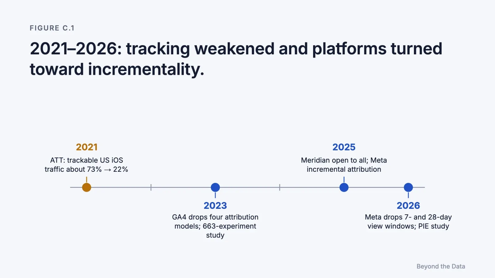
Appendix D · Test materials for Chapter 8
D.1 Prompt (version 3, cue-free), given verbatim
You are a marketing analyst. Below are six independent cases from six different online stores. For each case, tell the store owner what you would do. Use only the information given. Do not search the web.
Case 1. Last 30 days. Total ad spend €24,000: Meta €12,000, Google Ads €8,000, TikTok €4,000. Platform-reported revenue: Meta €49,200 (ROAS 4.1), Google Ads €28,800 (ROAS 3.6), TikTok €8,800 (ROAS 2.2). Total store revenue for the month (Shopify): €71,000. Contribution margin: 40%.
The owner wants to switch TikTok off and move its €4,000 to Meta, "because Meta's ROAS is almost twice TikTok's."
Case 2. Over the last 8 weeks the store ran a budget experiment. Each week, the budget of Channel X and the budget of Channel Y were each set at random, independently, to either €2,000 or €3,000. Average weekly store revenue:
| Weeks where… | Average weekly store revenue |
|---|---|
| X at €2,000 | €40,100 |
| X at €3,000 | €41,300 |
| Y at €2,000 | €39,300 |
| Y at €3,000 | €42,100 |
Platform-reported ROAS over the same period: Channel X 5.0, Channel Y 3.0. Half of revenue is profit before ad costs. Both channels now run at €2,500 a week.
The owner can add €1,000 a week to one channel and plans to give it to Channel X, "because X has the higher ROAS."
Case 3. Daily averages over the last month: Instagram spend €400, Google Search spend €600. Last-click report: Search 75 orders a day, Instagram 5, direct and organic 20. Store total: 100 orders a day. Each order brings €20 of profit before ad costs.
Two weeks ago the store paused Instagram in 4 of its 8 delivery regions, chosen by coin flip, for 14 days. During those 14 days the paused regions averaged 26 store orders a day in total, and the active regions averaged 51. In the 14 days before the pause, both groups averaged 50 orders a day. Search clicks in the paused regions also fell by about half.
The owner asks whether to switch Instagram off everywhere.
Case 4. Google Ads reports 300 conversions last month on €9,000 of spend. Each order brings €45 of profit before ad costs. Last quarter the store ran a randomised conversion-lift test on the same campaigns, which have not changed since. The test estimated that the ads caused 92% of the conversions Google reported (95% interval: 80% to 104%).
A consultant says: "Google always takes credit for sales that would have happened anyway. Switch Google Ads off."
Case 5. The store spends €5,000 a month on a YouTube campaign. The agency dashboard, using 7-day click attribution, shows €6,000 of YouTube revenue (ROAS 1.2). Half of revenue is profit before ad costs. Last spring the store switched YouTube off for 6 weeks in randomly chosen regions and compared total store revenue. That test estimated YouTube's incremental revenue at €15,000 per €5,000 of spend, mostly arriving 2 to 5 weeks after exposure. The campaign and targeting have not changed since.
The agency recommends cutting YouTube "because a ROAS of 1.2 is below your break-even of 2.0."
Case 6. The store spends €2,000 a month on retargeting website visitors. The platform's audience report says visitors who saw a retargeting ad converted at 4.0% within 30 days, while visitors who did not see one converted at 1.0%.
The agency proposes doubling the budget because retargeting "quadruples the conversion rate."
Answer format. For each case, write two or three sentences addressed to the owner. Start each answer with "Case N:".
D.2 Answer key and scoring rule
| Case | Correct decision | Reasoning |
|---|---|---|
| 1 | Do not move the budget; test incrementality first | Platform claims €86,800 exceed store revenue €71,000, so platform ROAS figures overlap and cannot rank channels |
| 2 | Give the extra €1,000 to Y | X: +€1,200 revenue → €600 profit < €1,000. Y: +€2,800 → €1,400 profit > €1,000 |
| 3 | Keep Instagram | Paused 50→26 (−24), active 50→51 (+1); effect −25 in half the store → about −50 orders a day store-wide × €20 = €1,000 > €400 |
| 4 | Keep Google Ads | 0.92 × 300 = 276 × €45 = €12,420 > €9,000; low end 240 × €45 = €10,800 > €9,000 |
| 5 | Keep YouTube | Incremental ROAS 3.0 > break-even 2.0 |
| 6 | Do not scale; run a holdout first | The 4× gap can come from targeting selection |
Scoring: in cases 1 and 6, an answer is correct only if it rejects the proposal and recommends an incrementality test before deciding; cautioning and then accepting the proposal is wrong. In cases 3 and 5, "increase" scores half a point. In case 4, "keep" and "increase" are correct.
Appendix E · Method of this book
Source selection. Peer-reviewed articles, working papers from recognised series (NBER, arXiv, SSRN), platforms' own documentation, and industry reports. Management magazines may inform framing but are never a source of numbers. A number enters the text only from a source whose abstract or full text was read; second-hand figures were traced to the original or dropped. The one exception is Lodish et al. (1995): its average elasticity and significance figures are given as reported in the working paper of Shapiro et al. (2021), whose full text was consulted, and the text says so.
Labels. Every claim carries an evidence label (Experiment, Observational, Model, Platform, Experiment vs observational, Analytical, Methodological review, Textbook principle, Industry survey, Benchmark, Our test, Our reading). Inferences are marked as "Our reading".
Platform sources. When a source is written by platform employees or uses platform data, this is noted at the citation.
Conflict of interest. The author is a co-founder of Meerkads, which builds advertising analytics software, including tools that let AI assistants read advertising data. No Meerkads data or product is used or described in this book.
Version. First edition, November 2026. Corrections will be listed with the date of change.
Appendix F · Formulas
This appendix collects the arithmetic behind the examples. Notation: R is revenue, S ad spend, Q orders or sales, m profit before ad costs as a share of revenue, and p profit per order.
F.1 Lift and incremental outcome (Chapters 4 and 5)
- Lift = (test average − control average) ÷ control average, where each average is the outcome per person or per region in that group.
- Incremental outcome = (test average − control average) × number of people or regions in the test group.
F.2 Incremental return and break-even (Chapters 5 and 6)
- iROAS = incremental revenue ÷ spend.
- Profit after ad costs = m × incremental revenue − S. Break-even iROAS = 1 ÷ m.
- With orders as the outcome: profit = p × incremental orders − S; break-even orders = S ÷ p.
- Examples: YouTube, m = 0.5, break-even 2.0, iROAS 15,000 ÷ 5,000 = 3.0, profit 0.5 × 15,000 − 5,000 = €2,500 a month (Chapter 6). Instagram, break-even 400 ÷ 20 = 20 orders a day (Chapter 5).
F.3 Difference in differences (Chapter 5)
- Effect = (test during − test before) − (control during − control before).
- Example: (46 − 50) − (51 − 50) = −5 orders a day.
- Assumption: without the change, both groups would have moved in parallel.
F.4 Scaling a partial test (Chapter 5)
- Whole-business effect = test effect ÷ k, where k is the test regions' share of the business, measured in orders before the test.
- Example: k = 0.5, so −5 ÷ 0.5 = −10 orders a day.
- Assumption: the effect is proportional to size, and the test regions are representative.
F.5 Standard error and 95% interval (Chapters 5 and 6)
- An average of n independent observations with standard deviation σ has standard error SE = σ ÷ √n.
- A difference between two independent estimates has SE = √(SE₁² + SE₂²).
- 95% interval ≈ estimate ± 1.96 × SE. With few observations, replace 1.96 by the t-value for the available degrees of freedom: 2.57 for 5.
- A count of independent events with mean μ has standard deviation √μ (Poisson).
- Geo example: daily gap SD = √(50 + 50) = 10; SE of each 14-day average gap = 10 ÷ √14 = 2.67; SE of the effect = √(2.67² + 2.67²) = 3.78; interval −5 ± 7.4 in the paused half, then × 2 for the whole store.
- Budget example: SE = 500 × √(1/4 + 1/4) = €354; for Y − X, SE = √(354² + 354²) = €500.
- Lift-test example: the interval on the caused share scales the count, 300 × 0.80 = 240 and 300 × 1.04 = 312 orders (Chapter 6).
F.6 How long a geo test must run (Chapter 5)
- With n days before and n days during, the half-width of the 95% interval for a difference in differences is h = 1.96 × σ × √(2 ÷ n), so n = 2 × (1.96 × σ ÷ h)².
- Example: σ = 10, n = 42 gives h = 4.3 orders in the paused half, 8.6 for the whole store, about ±€171 a day at €20 an order.
- With 8 regions there are 70 ways to choose 4. A randomisation test that compares the actual split with all of them cannot give a one-sided p-value below 1 ÷ 70 ≈ 0.014.
F.7 Average and marginal return (Chapter 6)
- Average ROAS = R ÷ S.
- Marginal return ≈ Δ*R* ÷ Δ*S* for a change Δ*S* in spend.
- Profit from each extra euro = m × Δ*R* ÷ Δ*S* − 1.
- Example: X, 0.5 × 1,200 ÷ 1,000 − 1 = −0.4; Y, 0.5 × 2,800 ÷ 1,000 − 1 = +0.4; that is −€400 and +€400 per extra €1,000.
F.8 Elasticity (Chapter 1)
- ε = (Δ*Q* ÷ Q) ÷ (Δ*S* ÷ S), the percentage change in sales for a 1% change in advertising.
- Example: ε = 0.12 and a 10% budget increase give about 0.12 × 10% = 1.2% more sales.
F.9 Carryover and diminishing returns (Chapters 6 and 7)
- Carryover (adstock), in a common form: *a*ₜ = *x*ₜ + λ × *a*ₜ₋₁, with 0 ≤ λ < 1, where *x*ₜ is this period's spend. Part of past spend still works this period.
- Shape: sales respond to f(a), a curve that rises ever more slowly. For such a curve starting at zero, the marginal return f′(a) is below the average f(a) ÷ a.
- Jin et al. (2017) use more general versions of both.
F.10 Shapley value (Chapter 3)
- For channel i among n channels, with v(T) the extra sales when only the channels in set T advertise: φᵢ = Σ over sets T without i of [|T|! × (n − |T| − 1)! ÷ n!] × [v(T with i) − v(T)].
- With two channels, this is the average of a channel's contribution when it comes first and when it comes second.
- Chapter 3 example, counting units above the 20 sold without advertising: v(none) = 0, v(Instagram) = 10, v(Search) = 30, v(both) = 80. Instagram: ½ × 10 + ½ × (80 − 30) = 30. Search: ½ × 30 + ½ × (80 − 10) = 50. The shares sum to 80, while switching each channel off loses 50 and 70. The split rests on assumptions about how the interaction is shared.
Practical guides
This page gathers, chapter by chapter, the Meerkads blog guides that describe the day-to-day practice of the topics in this book. The guides are not part of the book's chain of evidence; no claim in the book rests on them. The author's relationship to Meerkads is stated in the conflict-of-interest note in the front matter.
Chapter 1 · Why is the effect of advertising so hard to see?
Our earlier guides explain how platform figures differ from store revenue and how blended ROAS is calculated.
Chapter 2 · What does a reported conversion actually record?
Our step-by-step guides cover why Meta and Shopify revenue differ and how to compute True and Blended ROAS.
- Why your Meta Ads dashboard and Shopify revenue never match
- How to connect ad spend to actual store revenue
- Why your Facebook Ads ROAS is misleading you
- True ROAS vs Blended ROAS
Chapter 3 · What can an attribution model tell you, and what can't it?
Our earlier guides explain last touch in day-to-day reporting and how Performance Max reports credit.
Chapter 4 · Why do observational ad measurements overstate effects?
Our guides on detecting anomalies, creative fatigue, audience saturation and leading KPIs help locate changes before testing their causes.
- Ad attribution anomalies
- Creative fatigue in paid ads
- Audience saturation in paid social
- Facebook Ads KPIs that predict results
- Shopify analytics: the metrics that matter
Chapter 6 · How should budget follow evidence?
Our guide to audience saturation describes the signs that a channel's margin is falling.
Chapter 7 · How do attribution, experiments and models fit together?
Our guides on agency dashboards and PPC report templates describe the weekly reporting routine this system plugs into.
 Edip Ali Avcıbaşı · Co-founder & CAOCo-founder and CAO of Meerkads and Byte Digital. Has run agency operations since 2020, with a background in digital marketing, SEO and marketplaces.