
On this page 7 sections
Key findings
- For more than 80% of 288 TV-advertising brands, the marginal return was negative, even though the overall return was positive for about a third of them (Shapiro et al., 2021). [Observational]
- Attribution credit is proportional to a medium's marginal effectiveness multiplied by its past exposure; the profit-maximising budget does not depend on past exposure (Danaher & van Heerde, 2018). [Model]
- When two media reinforce each other, the optimal response is to raise total spend and shift some budget toward the less effective medium (Naik & Raman, 2003). [Model, market data]
- In media mix models, the estimated optimal mix can vary widely because the underlying parameters are uncertain (Jin et al., 2017). [Model]
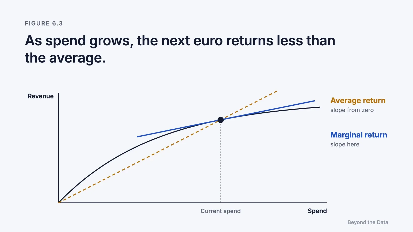
Short answer. Budget should follow the marginal return: what the next euro in a channel adds to total profit. Average return on ad spend, the number most reports show, describes the euros already spent. Saturation makes the margin lower than the average, delayed effects make short windows understate it, and synergy means a channel's margin depends on the others. When the evidence is weak, the best decision is often to keep the current budget and test.
What is the difference between average and marginal return?
The average return on ad spend divides all the revenue credited to a channel by all the money spent on it. The marginal return is the extra profit from the next unit of spend. Budget decisions are always about the next unit: whether to add, cut or move money. The average is therefore the wrong number for the decision, even when it is measured correctly.
An experiment from the test in Chapter 8 shows how far the two can diverge.
Over 8 weeks, a store set the weekly budgets of Channel X and Channel Y at random, each to either €2,000 or €3,000. Average weekly store revenue:
| Weeks where | Revenue |
|---|---|
| X at €2,000 | €40,100 |
| X at €3,000 | €41,300 |
| Y at €2,000 | €39,300 |
| Y at €3,000 | €42,100 |
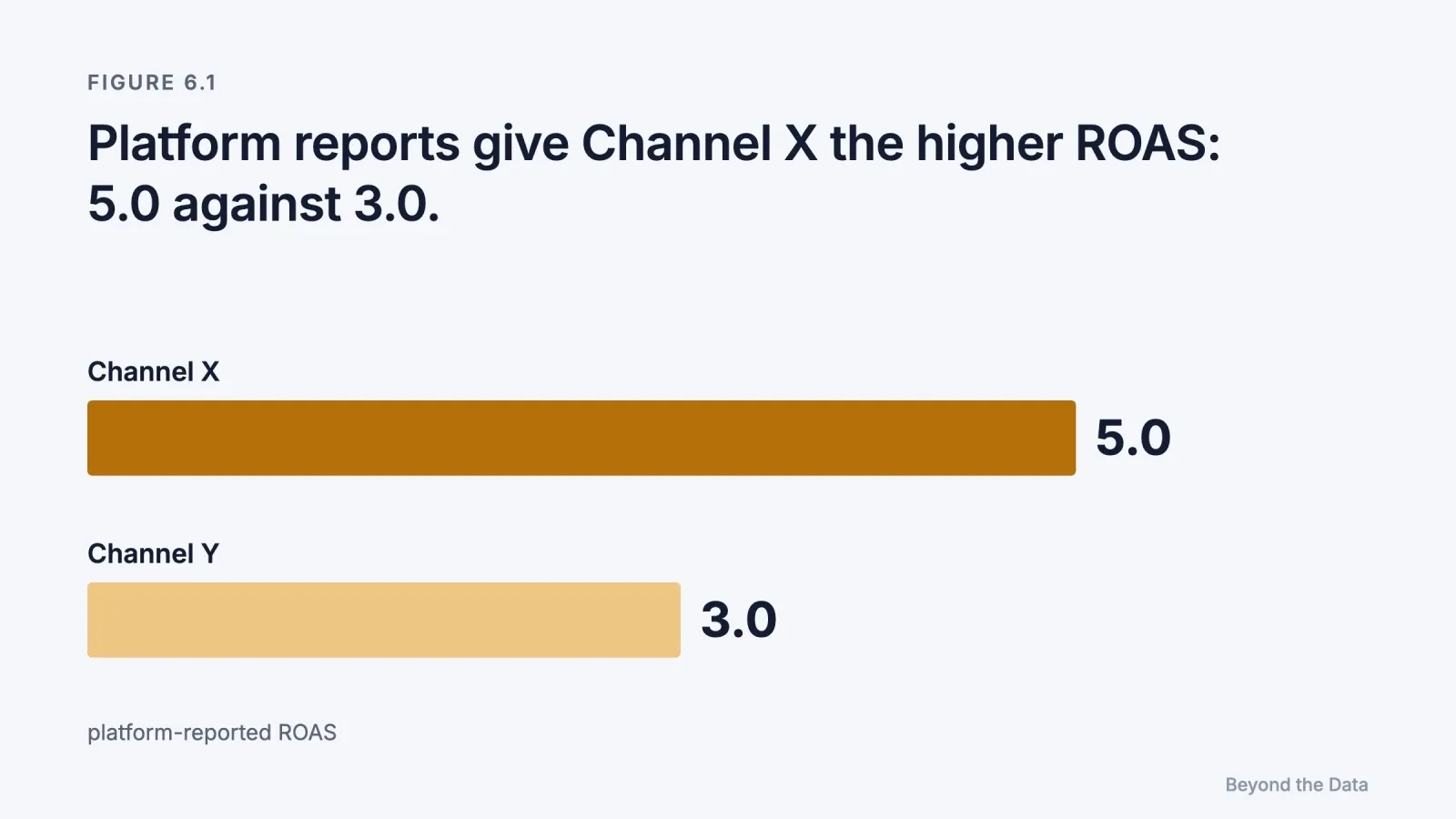
Platform-reported ROAS: X 5.0, Y 3.0. Half of revenue is profit before ad costs.
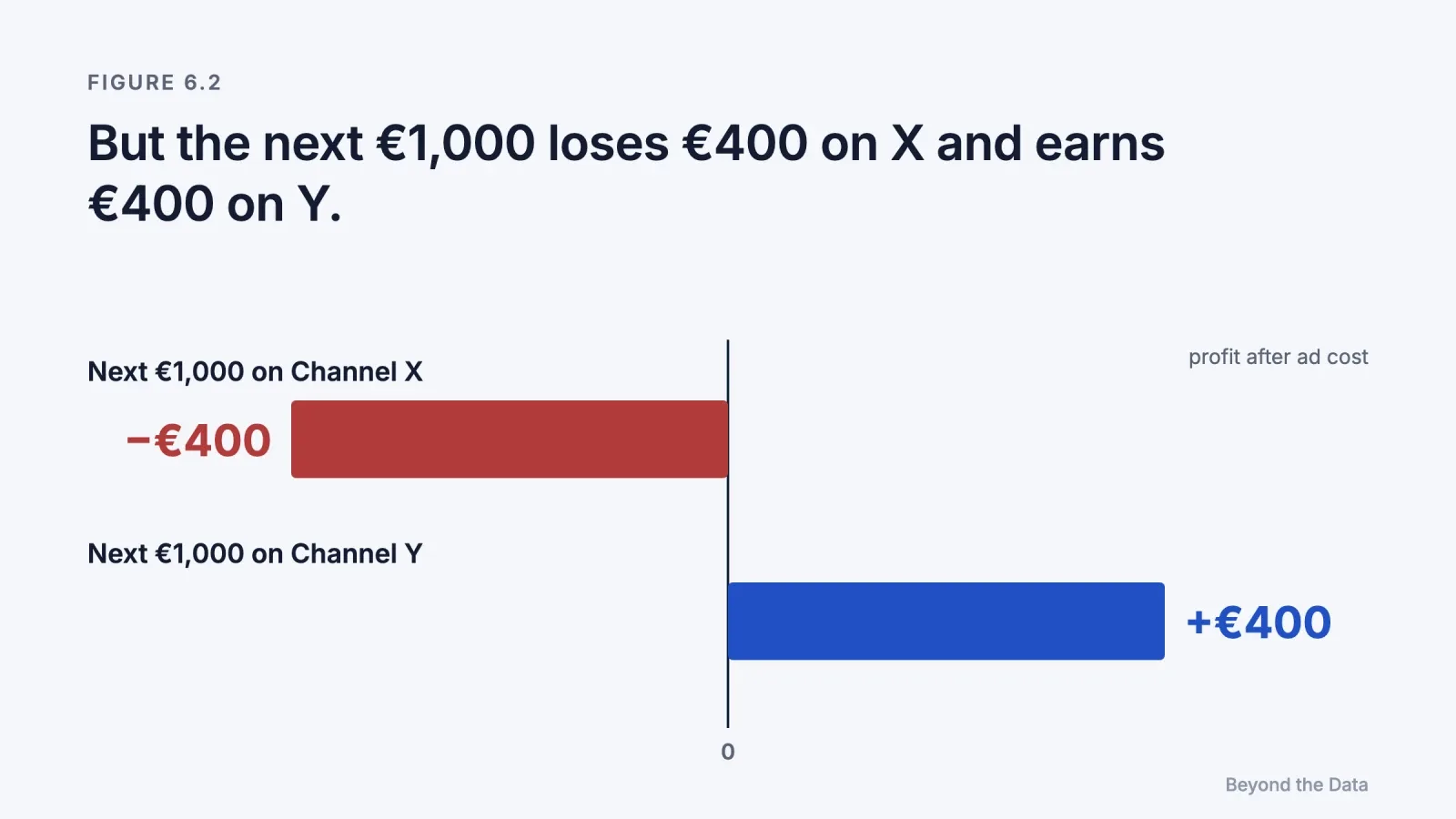
- Extra €1,000 on X: +€1,200 revenue → +€600 profit → €400 loss after the spend
- Extra €1,000 on Y: +€2,800 revenue → +€1,400 profit → €400 gain
Illustrative example.
The channel with the higher average return is the worse place for the next euro. This is the normal situation for a channel that has been scaled up: its best audiences were reached first, so its average stays high while its margin falls.
How sure is that ranking? Suppose each of the four budget combinations fell in 2 of the 8 weeks, and weekly revenue varies around its expected level with a standard deviation of €500. Each channel's effect then compares 4 weeks with 4 weeks:
- Standard error of each channel's effect: €500 × √(1/4 + 1/4) ≈ €354, so the 95% interval is about ±€690
- X: +€1,200 of revenue (€510 to €1,890) → between about −€750 and −€50 after the extra spend
- Y: +€2,800 of revenue (€2,110 to €3,490) → between about +€50 and +€750 after the extra spend
- Y minus X: +€1,600 of revenue, standard error €500 → €620 to €2,580
With only 8 weeks of data, an interval based on the t-distribution, which multiplies by 2.57 instead of 1.96, is about 30% wider. Y's own gain could then fall slightly below zero, while Y still beats X. The ranking is more certain than the profit. The €500 is an illustrative assumption; Case 2 of the test gives only the averages.
Why does the margin fall as spend rises?
Because of saturation. The first euros in a channel reach the most responsive audiences at the lowest cost. Additional euros reach people who are less interested, more expensive to reach, or already reached. Media mix models capture this with a shape (diminishing-returns) curve (Jin et al., 2017).
Shapiro and colleagues' results on 288 brands show how much it matters. For most brands, the last dollar of TV advertising returned less than it cost, even though the advertising as a whole was profitable for about a third of them (Shapiro et al., 2021). [Our reading] Even in the third of brands where advertising paid overall, an advertiser reading only the average return would conclude that the channel works and would keep scaling it past the point where it pays.
How do delayed effects distort the picture?
Advertising often works with a delay. Someone sees a video today and buys in three weeks. Attribution windows of 1 or 7 days miss this, so channels whose effects arrive late look weaker than they are. Media mix models represent the delay as carryover, or adstock, a decaying effect that continues after the spend (Jin et al., 2017).
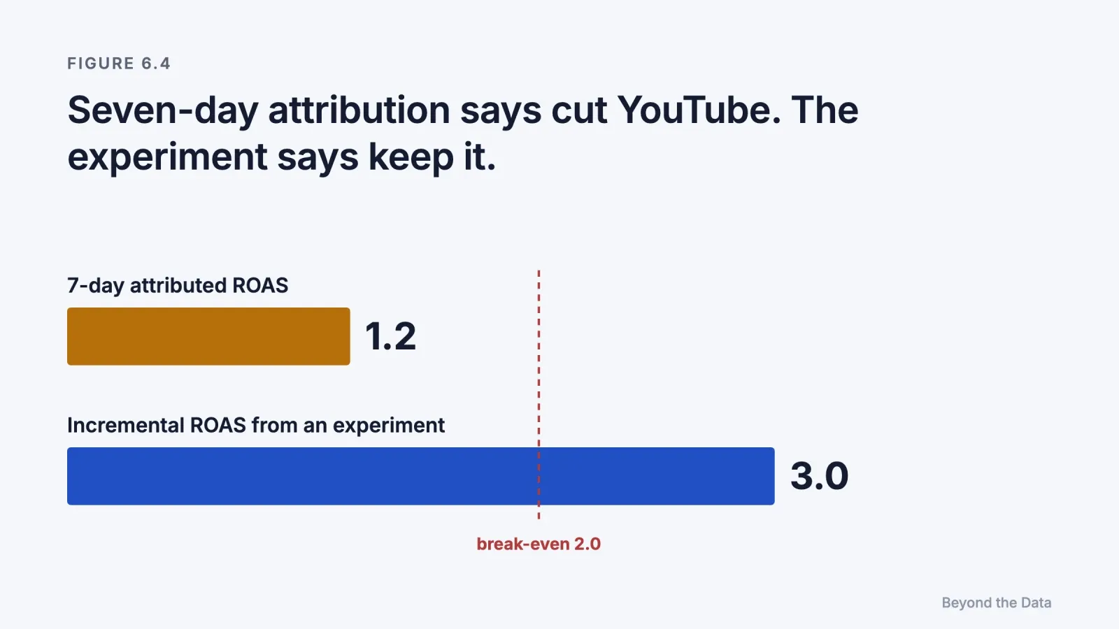
A store spends €5,000 a month on YouTube. The agency dashboard, with 7-day click attribution, shows €6,000 of revenue (ROAS 1.2). Half of revenue is profit, so break-even ROAS is 2.0. A regional experiment last spring estimated €15,000 of incremental revenue per €5,000 of spend (95% interval €10,500 to €19,500), mostly arriving 2 to 5 weeks after exposure.
- Attributed ROAS: 1.2, below break-even → "cut it"
- Incremental ROAS: 3.0, above break-even → about €2,500 a month of profit after ad costs
- Low end of the interval: ROAS 2.1, still above break-even → about €250 a month
Illustrative example used in the test in Chapter 8. The interval is added here; Case 5 of the test gives only the estimate.
The same campaign looks unprofitable or profitable depending on whether the measurement window covers the delay.
How does synergy change the decision?
If channels reinforce each other, as Chapter 3 showed for display and search, a channel's margin depends on how much is spent on the others. Naik and Raman (2003) estimated synergy between TV and print in Dockers' advertising and derived a counterintuitive rule: as synergy rises, an advertiser should spend more in total and shift some budget toward the less effective medium, because that medium increases the return on the more effective one. [Model, market data]
Attribution cannot capture this rule. It assigns each channel a fixed share, while the true value of each channel changes with the others' budgets. Danaher and van Heerde (2018) make a related point in a paper titled "Delusion in Attribution": attribution credit reflects a medium's marginal effectiveness multiplied by its past exposure, while the profit-maximising allocation does not depend on past exposure at all. Allocating by attribution shares therefore tends to reproduce last year's plan.
What should you do when the evidence is uncertain?
Treat the decision as a choice under uncertainty, and price the uncertainty. [Our reading]
| Situation | Evidence available | Typical correct decision |
|---|---|---|
| A trusted experiment shows the channel is profitable, even at the low end of its interval | Experiment, interval above break-even | Keep, whatever attribution says |
| Attribution and an experiment disagree | Experiment and attribution | Follow the experiment, then check whether the attribution window misses delayed effects |
| Two channels compete for one budget increase and a budget-level test exists | Marginal returns from a test | Give the money to the higher marginal return, not the higher average |
| Only attribution exists and platform claims overlap | Attribution only | Keep the budget unchanged and run a test before cutting or scaling |
| Exposed users convert much more than unexposed ones | Observational comparison only | Do not scale on that gap; run a holdout first |
The last two rows deserve emphasis. When the only evidence is attribution, switching a channel off can destroy value that the reports never showed, and scaling a channel can pour money into selection. A short test is usually cheaper than either mistake. The value of a test is the expected loss from the decision it prevents.
An example from Chapter 8's test illustrates the first row.
Google Ads reports 300 conversions on €9,000 of spend; each order brings €45 of profit. A randomised lift test on the same campaigns found that 92% of reported conversions were caused by the ads (95% interval 80–104%).
- Central estimate: 276 incremental orders × €45 = €12,420 profit → about €3,420 above spend
- Low end: 240 orders × €45 = €10,800 → still about €1,800 above spend
A consultant's general claim that "Google takes credit for sales that would have happened anyway" is true in many settings and false here.
Discounting every platform number by a fixed amount is as much of a shortcut as trusting every platform number. The evidence on each channel decides.
The limit of this chapter
Every rule in this chapter needs a response curve for each channel: how returns change with spend, how long they take to arrive, and how they depend on other channels. Experiments supply a few points on those curves. To estimate the whole set together, an advertiser needs a model of all channels at once, and a way to keep it honest. Chapter 7 describes how attribution, experiments and models fit together.
References
- Danaher, P. J., & van Heerde, H. J. (2018). Delusion in attribution: Caveats in using attribution for multimedia budget allocation. Journal of Marketing Research, 55(5), 667–685. doi:10.1177/0022243718802845
- Jin, Y., Wang, Y., Sun, Y., Chan, D., & Koehler, J. (2017). Bayesian methods for media mix modeling with carryover and shape effects. Google Inc.
- Naik, P. A., & Raman, K. (2003). Understanding the impact of synergy in multimedia communications. Journal of Marketing Research, 40(4), 375–388. doi:10.1509/jmkr.40.4.375.19385
- Shapiro, B. T., Hitsch, G. J., & Tuchman, A. E. (2021). TV advertising effectiveness and profitability: Generalizable results from 288 brands. Econometrica, 89(4), 1855–1879. doi:10.3982/ECTA17674
 Edip Ali Avcıbaşı · Co-founder & CAOCo-founder and CAO of Meerkads and Byte Digital. Has run agency operations since 2020, with a background in digital marketing, SEO and marketplaces.